We take a top-down approach to introducing reinforcement learning (RL) by starting with a toy example: a student going through college. In order to frame the problem from the RL point-of-view, we’ll walk through the following steps:
- Setting up a model of the problem as a Markov Decision Process, the framework that underpins the RL approach to sequential decision-making problems
- Deciding on an objective: maximize rewards
- Writing down an equation whose solution is our objective: Bellman equations
David Silver walks through this example in his lecture notes on RL, but as far as we can tell, does not provide code, so we’re sharing our implementation, comprising:
- the student’s college environment using the OpenAI gym package.
- a jupyter notebook sampling from the model
Student in toy college
We model the student as an agent in a college environment who can move between five states: CLASS 1, 2, 3, the FACEBOOK state, and SLEEP state. The states are represented by the four circles and square. The SLEEP state — the square with no outward bound arrows — is a terminal state, i.e. once a student reaches that state, her journey is finished.
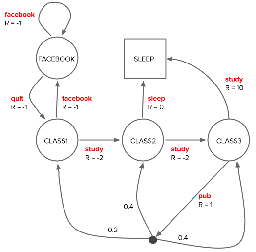
Actions that a student can take in her current state are labeled in red (facebook/quit/study/sleep/pub) and influence which state she’ll find herself in next.
In this model, most state transitions are deterministic functions of the action in the current state, e.g. if she decides to study in CLASS 1, then she’ll definitely advance to CLASS 2. The single non-deterministic state transition is if she goes pubbing while in CLASS 3, where the pubbing action is indicated by a solid dot; she can end up in CLASS 1, 2 or back in 3 with probability 0.2, 0.4, or 0.4, respectively, depending on how reckless the pubbing was.
The model also specifies the reward \(R\) associated with acting in one state and ending up in the next. In this example, the dynamics \(p(s’,r|s,a)\), are given to us, i.e. we have a full model of the environment, and, hopefully, the rewards have been designed to capture the actual end goal of the student.
Markov Decision Process
Formally, we’ve modeled the student’s college experience as a finite Markov Decision Process (MDP). The dynamics are Markov because the probability of ending up in the next state depends only on the current state and action, not on any history leading up to the current state. The Markov property is integral to the simplification of the equations that describe the model, which we’ll see in a bit.
The components of an MDP are:
- \(S\) - the set of possible states
- \(R\) - the set of (scalar) rewards
- \(A\) - the set of possible actions in each state
The dynamics of the system are described by the probabilities of receiving a reward in the next state given the current state and action taken, \(p(s’,r|s,a)\). In this example, the MDP is finite because there are a finite number of states, rewards, and actions.
The student’s agency in this environment comes from how she decides to act in each state. The mapping of a state to actions is the policy, \(\pi(a|s) := p(a|s)\), and can be a deterministic or stochastic function of her state.
Suppose we have an indifferent student who always chooses actions randomly. We can sample from the MDP to get some example trajectories the student might experience with this policy. In the sample trajectories below, the states are enclosed in parentheses (STATE), and actions enclosed in square brackets [action].
Sample trajectories:
(CLASS1)--[facebook]-->(FACEBOOK)--[facebook]-->(FACEBOOK)--[facebook]-->(FACEBOOK)--[facebook]-->(FACEBOOK)--[quit]-->(CLASS1)--[facebook]-->(FACEBOOK)--[quit]-->(CLASS1)--[study]-->(CLASS2)--[sleep]-->(SLEEP)

(FACEBOOK)--[quit]-->(CLASS1)--[study]-->(CLASS2)--[study]-->(CLASS3)--[study]-->(SLEEP)

(SLEEP)

(CLASS1)--[facebook]-->(FACEBOOK)--[quit]-->(CLASS1)--[study]-->(CLASS2)--[sleep]-->(SLEEP)

(FACEBOOK)--[facebook]-->(FACEBOOK)--[facebook]-->(FACEBOOK)--[facebook]-->(FACEBOOK)--[facebook]-->(FACEBOOK)--[quit]-->(CLASS1)--[facebook]-->(FACEBOOK)--[quit]-->(CLASS1)--[study]-->(CLASS2)--[study]-->(CLASS3)--[pub]-->(CLASS2)--[study]-->(CLASS3)--[study]-->(SLEEP)
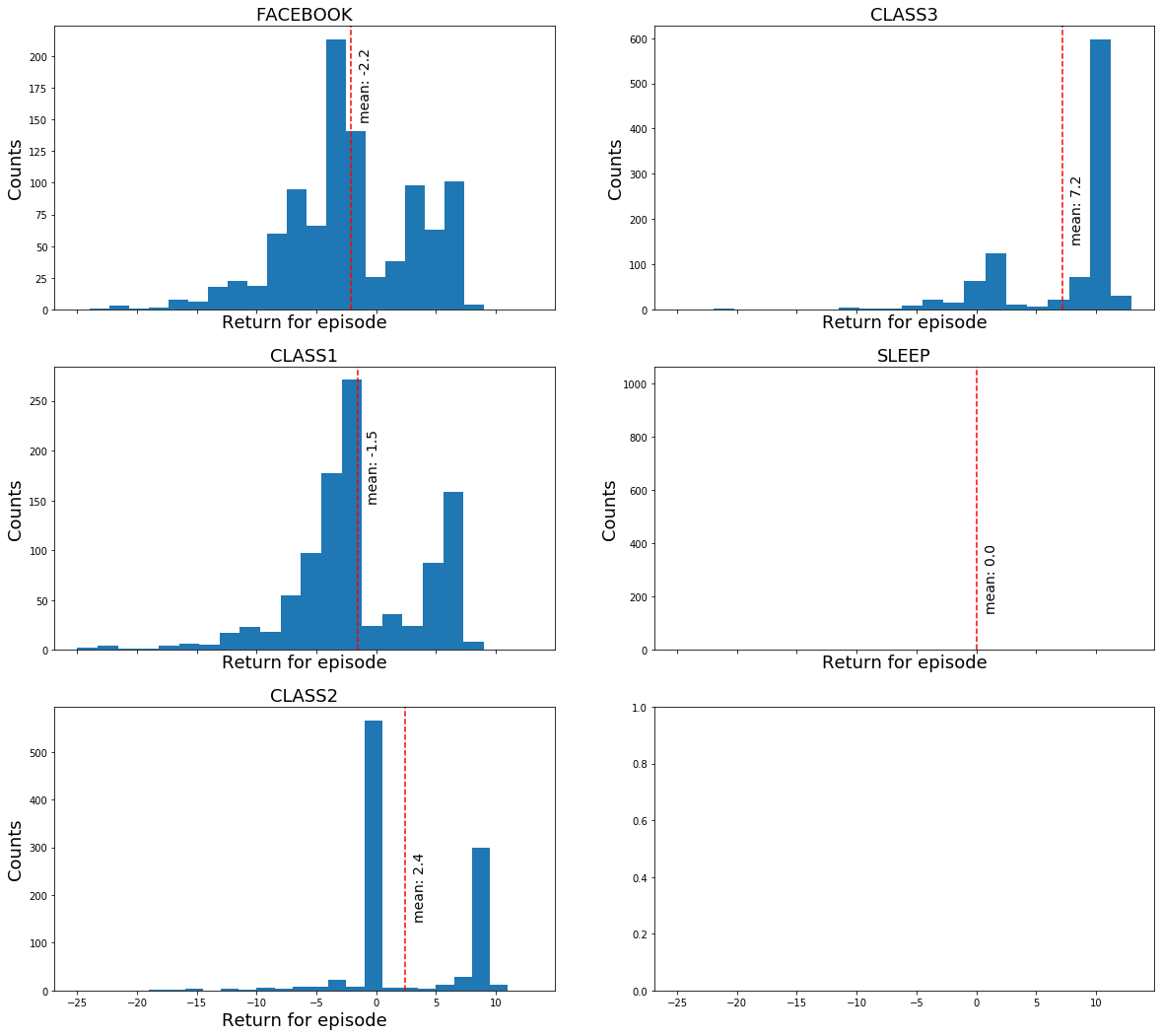
Rewards following a random policy:
Under this random policy, what total reward would the student expect when starting from any of the states? We can estimate the expected rewards by summing up the rewards per trajectory and plotting the distributions of total rewards per starting state:
Maximizing rewards: discounted return and value functions
We’ve just seen how we can estimate rewards starting from each state given a random policy. Next, we’ll formalize our goal in terms of maximizing returns.
Returns
We simply summed the rewards from the sample trajectories above, but the quantity we often want to maximize in practice is the discounted return \(G_t\), which is a sum of the weighted rewards:
where \(0 \leq \gamma \leq 1\). \(\gamma\) is the discount rate which characterizes how much we weight rewards now vs. later. Discounting is mathematically useful for avoiding infinite returns in MDPs without a terminal state and allows us to account for uncertainty in the future when we don’t have a perfect model of the environment.
Aside
The discount factor introduces a time scale since it says that we don’t care about rewards that are far in the future. The half-life (actually, the \(1/e\) life) of a reward in units of time steps is \(1/(1-\gamma)\), which comes from a definition of \(1/e\):
\(\gamma = 0.99\) is often used in practice, which corresponds to a half-life of 100 timesteps since \(0.99^{100} = (1 - 1/100)^{100} \approx 1/e\).
Value functions
Earlier, we were able to estimate the expected undiscounted returns starting from each state by sampling from the MDP under a random policy. Value functions formalize this notion of the “goodness” of being in a state.
State value function \(v\)
The state value function \(v_{\pi}(s)\) is the expected return when starting in state \(s\), following policy \(\pi\).
The state value function can be written as a recursive relationship, the Bellman expectation equation, expressing the value of a state in terms of the values of its neighors by making use of the Markov property.
This equation expresses the value of a state as an average over the discounted value of its neighbor / successor states, plus the expected reward transitioning from \(s\) to \(s’\), and \(v_{\pi}\) is the unique* solution. The distribution of rewards depends on the student’s policy since her actions influence her future rewards.
Note on terminology: Policy evaluation uses the Bellman expectation equation to solve for the value function given a policy \(\pi\) and environment dynamics \(p(s’, r | s, a)\). This is different from policy iteration and value iteration, which are concerned with finding an optimal policy.
We can solve the Bellman equation for the value function as an alternative to the sampling we did earlier for the student toy example. Since the problem has a small number of states and actions, and we have full knowledge of the environment, an exact solution is feasible by directly solving the system of linear equations or iteratively using dynamic programming. Here is the solution to (\ref{state-value-bellman}) for \(v\) under a random policy in the student example (compare to the sample means in the histogram of returns):
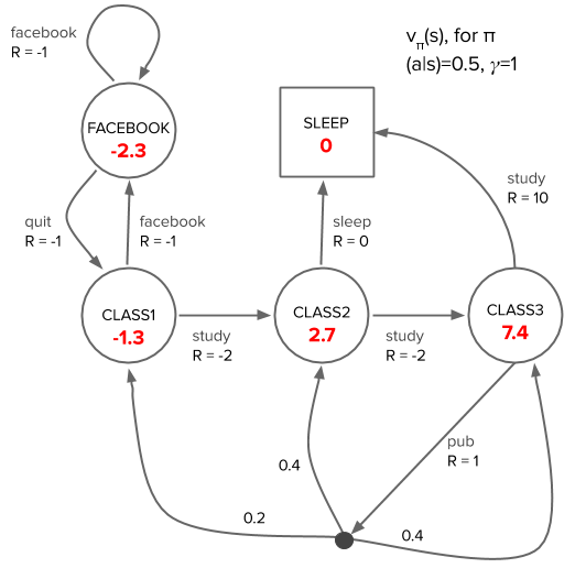
We can verify that the solution is self-consistent by spot checking the value of a state in terms of the values of its neighboring states according to the Bellman equation, e.g. the CLASS1 state with \(v_{\pi}(\text{CLASS1}) = -1.3\):
Action value function \(q\)
Another value function is the action value function \(q_{\pi}(s, a)\), which is the expected return from a state \(s\) if we follow a policy \(\pi\) after taking an action \(a\):
We can also write \(v\) and \(q\) in terms of each other. For example, the state value function can be viewed as an average over the action value functions for that state, weighted by the probability of taking each action, \(\pi\), from that state:
Rewriting \(v\) in terms of \(q\) in (\ref{state-value-one-step-backup}) is useful later for thinking about the “advantage”, \(A(s,a)\), of taking an action in a state, namely how much better is an action in that state than the average?
Why \(q\) in addition to \(v\)?
Looking ahead, we almost never have access to the environment dynamics in real world problems, but solving for \(q\) instead of \(v\) lets us get around this problem; we can figure out the best action to take in a state solely using \(q\) (we further expand on this in our discussion below on the Bellman optimality equation for \(q_*\).
A concrete example of using \(q\) is provided in our post on multiarmed bandits (an example of a simple single-state MDP), which discusses agents/algorithms that don’t have access to the true environment dynamics. The strategy amounts to estimating the action value function of the slot machine and using those estimates to inform which slot machine arms to pull in order to maximize rewards.
Optimal value and policy
The crux of the RL problem is finding a policy that maximizes the expected return. A policy \(\pi\) is defined to be better than another policy \(\pi’\) if \(v_{\pi}(s) > v_{\pi’}(s)\) for all states. We are guaranteed* an optimal state value function \(v_*\) which corresponds to one or more optimal policies \(\pi*\).
Recall that the value function for an arbitrary policy can be written in terms of an average over the action values for that state (\ref{state-value-one-step-backup}). In contrast, the optimal value function \(v_*\) must be consistent with following a policy that selects the action that maximizes the action value functions from a state, i.e. taking a \(\max\) (\ref{state-value-bellman-optimality}) instead of an average (\ref{state-value-one-step-backup}) over \(q\), leading to the Bellman optimality equation for \(v_*\):
The optimal policy immediately follows: take the action in a state that maximizes the right hand side of (\ref{state-value-bellman-optimality}). The principle of optimality, which applies to the Bellman optimality equation, means that this greedy policy actually corresponds to the optimal policy! Note: Unlike the Bellman expectation equations, the Bellman optimality equations are a nonlinear system of equations due to taking the max.
The Bellman optimality equation for the action value function \(q_*(s,a)\) is:
Looking ahead: In practice, without a knowledge of the environment dynamics, RL algorithms based on solving value functions can approximate the expectation in (\ref{action-value-bellman-optimality}) by sampling, i.e. interacting with the environment, and iteratively selecting the action that corresponds to maximizing \(q\) in each state that the agent lands in along its trajectory, which is possible since the maximum occurs inside the summation in (\ref{action-value-bellman-optimality}). In contrast, this sampling approach doesn’t work for (\ref{state-value-bellman-optimality}) because of the maximum outside the summation in…that’s why action value functions are so useful when we lack a model of the environment!
Here is the optimal state value function and policy for the student example, which we solve for in a later post:
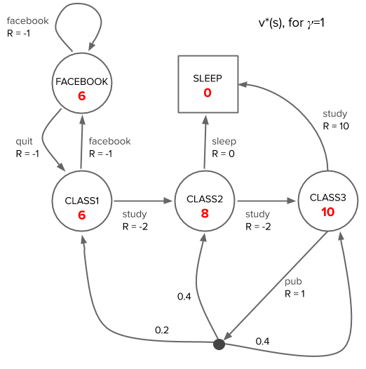
Comparing the values per state under the optimal policy vs the random policy, the value in every state under the optimal policy exceeds the value under the random policy.
Summary
We’ve discussed how the problem of sequential decision making can be framed as an MDP using the student toy MDP as an example. The goal in RL is to figure out a policy — what actions to take in each state — that maximizes our returns.
MDPs provide a framework for approaching the problem by defining the value of each state, the value functions, and using the value functions to define what a “best policy” means. The value functions are unique solutions to the Bellman equations, and the MDP is “solved” when we know the optimal value function.
Much of reinforcement learning centers around trying to solve these equations under different conditions, e.g. unknown environment dynamics and large — possibly continuous — states and/or action spaces that require approximations to the value functions.
We’ll discuss how we arrived at the solutions for this toy problem in a future post!
Example code
Code for sampling from the student environment under a random policy in order to generate the trajectories and histograms of returns is available in this jupyter notebook.
The code for the student environment creates an environment with an API that is compatible with OpenAI gym — specifically, it is derived from the gym.envs.toy_text.DiscreteEnv environment.
The uniqueness of the solution to the Bellman equations for finite MDPs is stated without proof in Ref [2], but Ref [1] motivates it briefly via the contraction mapping theorem*.
References
[1] David Silver’s RL Course Lecture 2 - (video, slides)
[2] Sutton and Barto - Reinforcement Learning: An Introduction - Chapter 3: Finite Markov Decision Processes
 Cathy Yeh got a PhD at UC Santa Barbara studying soft-matter/polymer physics. After stints in a translational modeling group at Pfizer in San Diego, Driver (a no longer extant startup trying to match cancer patients to clinical trials) in San Francisco, and Square, she is currently participating in the OpenAI Scholars program.