Backpropagation in neural networks

Overview

We give a short introduction to neural networks and the backpropagation algorithm for training neural networks. Our overview is brief because we assume familiarity with partial derivatives, the chain rule, and matrix multiplication.

We also hope this post will be a quick reference for those already familiar with the notation used by Andrew Ng in his course on “Neural Networks and Deep Learning”, the first in the deeplearning.ai series on Coursera. That course provides but doesn’t derive the vectorized form of the backpropagation equations, so we hope to fill in that small gap while using the same notation.

Introduction: neural networks

A single neuron acting on a single training example

single neuron

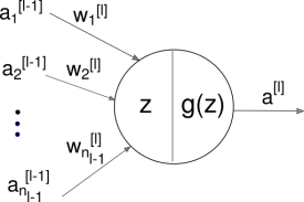
The basic building block of a neural network is the composition of a nonlinear function (like a sigmoid, tanh, or ReLU) \(g(z)\)

\begin{eqnarray} \nonumber a^{[l]} = g(z^{[l]}) \end{eqnarray}

with a linear function acting on a (multidimensional) input, \(a\).

\begin{eqnarray} \nonumber z^{[l]} = w^{[l]T} a^{[l-1]} + b^{[l]} \end{eqnarray}

These building blocks, i.e. “nodes” or “neurons” of the neural network, are arranged in layers, with the layer denoted by superscript square brackets, e.g. \([l]\) for the \(l\)th layer. \(n_l\) denotes the number of neurons in layer \(l\).

Forward propagation

Forward propagation is the computation of the multiple linear and nonlinear transformations of the neural network on the input data. We can rewrite the above equations in vectorized form to handle multiple training examples and neurons per layer as

\begin{eqnarray} \tag{1} \label{1} A^{[l]} = g(Z^{[l]}) \end{eqnarray}

with a linear function acting on a (multidimensional) input, \(A\).

\begin{eqnarray} \tag{2} \label{2} Z^{[l]} = W^{[l]} A^{[l-1]} + b^{[l]} \end{eqnarray}

The outputs or activations, \(A^{[l-1]}\), of the previous layer serve as inputs for the linear functions, \(z^{[l]}\). If \(n_l\) denotes the number of neurons in layer \(l\), and \(m\) denotes the number of training examples in one (mini)batch pass through the neural network, then the dimensions of these matrices are:

Variable	Dimensions
\(A^{[l]}\)	(\(n_l\), \(m\))
\(Z^{[l]}\)	(\(n_l\), \(m\))
\(W^{[l]}\)	(\(n_l\), \(n_{l-1}\))
\(b^{[l]}\)	(\(n_l\), 1)

For example, this neural network consists of only a single hidden layer with 3 neurons in layer 1.

neural network

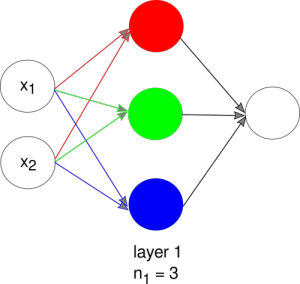
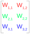
The matrix \(W^{[1]}\) has dimensions (3, 2) because there are 3 neurons in layer 1 and 2 inputs from the previous layer (in this example, the inputs are the raw data, \(\vec{x} = (x_1, x_2)\)). Each row of \(W^{[1]}\) corresponds to a vector of weights for a neuron in layer 1.

weights matrix

The final output of the neural network is a prediction in the last layer \(L\), and the closeness of the prediction \(A^{[L](i)}\) to the true label \(y^{(i)}\) for training example \(i\) is quantified by a loss function \(\mathcal{L}(y^{(i)}, A^{[L](i)})\), where superscript \((i)\) denotes the \(i\)th training example. For classification, the typical choice for \(\mathcal{L}\) is the cross-entropy loss (log loss).

The cost \(J\) is the average loss over all \(m\) training examples in the dataset.

\begin{eqnarray} \tag{3} \label{3} J = \frac{1}{m} \sum_{i=1}^m \mathcal{L}(y^{(i)}, A^{[L](i)}) \end{eqnarray}

Minimizing the cost with gradient descent

The task of training a neural network is to find the set of parameters \(W\) and \(b\) (with different \(W\) and \(b\) for different nodes in the network) that will give us the best predictions, i.e. minimize the cost (\ref{3}).

Gradient descent is the workhorse that we employ for this optimization problem. We randomly initialize the parameters \(W\) and \(b\) for each node, then iteratively update the parameters by moving them in the direction that is opposite to the gradient of the cost.

\begin{eqnarray} \nonumber W_\text{new} &=& W_\text{previous} - \alpha \frac{\partial J}{\partial W} \\ b_\text{new} &=& b_\text{previous} - \alpha \frac{\partial J}{\partial b} \end{eqnarray}

\(\alpha\) is the learning rate, a hyperparameter that needs to be tuned during the training process. The gradient of the cost is calculated by the backpropagation algorithm.

Backpropagation equations

These are the vectorized backpropagation (BP) equations which we wish to derive:

\begin{eqnarray} \nonumber dW^{[l]} &\equiv& \frac{\partial J}{\partial W^{[l]}} = \frac{1}{m} dZ^{[l]}A^{[l-1]T} \tag{BP1} \label{BP1} \\ db^{[l]} &\equiv& \frac{\partial J}{\partial b^{[l]}} = \frac{1}{m} \sum_{i=1}^m dZ^{[l](i)} \tag{BP2} \label{BP2} \\ dA^{[l-1]} &\equiv& \frac{\partial \mathcal{L}}{\partial A^{[l-1]}} = W^{[l]T}dZ^{[l]} \tag{BP3} \label{BP3} \\ dZ^{[l]} &\equiv& \frac{\partial \mathcal{L}}{\partial Z^{[l]}} = dA^{[l]} * g'(Z^{[l]}) \tag{BP4} \label{BP4} \end{eqnarray}

The \(*\) in the last line denotes element-wise multiplication.

\(W\) and \(b\) are the parameters we want to learn (update), but the BP equations include two additional expressions for the partial derivative of the loss in terms of linear and nonlinear activations per training example since they are intermediate terms that appear in the calculation of \(dW\) and \(db\).

Chain rule

We’ll need the chain rule for total derivatives, which describes how the change in a function \(f\) with respect to a variable \(x\) can be calculated as a sum over the contributions from intermediate functions \(u_i\) that depend on \(x\):

\begin{eqnarray} \nonumber \frac{\partial f(u_1, u_2, ..., u_k)}{\partial x} = \sum_{i}^k \frac{\partial f}{\partial u_i} \frac{\partial u_i}{\partial x} \end{eqnarray}

where the \(u_i\) are functions of \(x\). This expression reduces to the single variable chain rule when only one \(u_i\) is a function of \(x\).

The gradients for every node can be calculated in a single backward pass through the network, starting with the last layer and working backwards, towards the input layer. As we work backwards, we cache the values of \(dZ\) and \(dA\) from previous calculations, which are then used to compute the derivative for variables that are further upstream in the computation graph. The dependency of the derivatives of upstream variables on downstream variables, i.e. cached derivatives, is manifested in the \(\frac{\partial f}{\partial u_i}\) term in the chain rule. (Backpropagation is a dynamic programming algorithm!)

The chain rule applied to backpropagation

In this section, we apply the chain rule to derive the vectorized form of equations BP(1-4). Without loss of generality, we’ll index an element of the matrix or vector on the left hand side of BP(1-4); the notation for applying the chain rule is therefore straightforward because the derivatives are just with respect to scalars.

BP1 The partial derivative of the cost with respect to the \(s\)th component (corresponding to the \(s\)th input) of \(\vec{w}\) in the \(r\)th node in layer \(l\) is:

\begin{eqnarray} dW^{[l]}_{rs} &\equiv& \frac{\partial J}{\partial W^{[l]}_{rs}} \\ &=& \frac{1}{m} \sum_{i}^m \frac{\partial \mathcal{L}}{\partial W^{[l]}_{rs}} \\ &=& \frac{1}{m} \sum_{i}^m \frac{\partial \mathcal{L}}{\partial z^{[l]}_{ri}} \frac{\partial z^{[l]}_{ri}}{\partial W^{[l]}_{rs}} \tag{4} \label{4} \end{eqnarray}

The last line is due to the chain rule.

The first term in (\ref{4}) is \(dZ^{[l]}_{ri}\) by definition (\ref{BP4}). We can simplify the second term of (\ref{4}) using the definition of the linear function (\ref{2}), which we rewrite below explicitly for the \(i\)th training example in the \(r\)th node in the \(l\)th layer in order to be able to more easily keep track of indices when we take derivatives of the linear function:

\begin{eqnarray} \tag{5} \label{5} Z^{[l]}_{ri} = \sum_j^{n_{l-1}} W^{[l]}_{rj} A^{[l-1]}_{ji} + b^{[l]}_r \end{eqnarray}

where \(n_{l-1}\) denotes the number of nodes in layer \(l-1\).

Therefore,

\begin{eqnarray} dW^{[l]}_{rs} &=& \frac{1}{m} \sum_{i}^m dZ^{[l]}_{ri} A^{[l-1]}_{si} \\ &=& \frac{1}{m} \sum_{i}^m dZ^{[l]}_{ri} A^{[l-1]T}_{is} \\ &=& \frac{1}{m} \left( dZ^{[l]} A^{[l-1]T} \right)_{rs} \end{eqnarray}

BP2 The partial derivative of the cost with respect to \(b\) in the \(r\)th node in layer \(l\) is:

\begin{eqnarray} db^{[l]}_r &\equiv& \frac{\partial J}{\partial b^{[l]}_r} \\ &=& \frac{1}{m} \sum_{i}^m \frac{\partial \mathcal{L}}{\partial b^{[l]}_r} \\ &=& \frac{1}{m} \sum_{i}^m \frac{\partial \mathcal{L}}{\partial z^{[l]}_{ri}} \frac{\partial z^{[l]}_{ri}}{\partial b^{[l]}_r} \tag{6} \label{6} \\ &=& \frac{1}{m} \sum_{i}^m dZ^{[l]}_{ri} \end{eqnarray}

(\ref{6}) is due to the chain rule. The first term in (\ref{6}) is \(dZ^{[l]}_{ri}\) by definition (\ref{BP4}). The second term of (\ref{6}) simplifies to \(\partial z^{[l]}_{ri} / \partial b^{[l]}_r = 1\) from (\ref{5}).

BP3 The partial derivative of the loss for the \(i\)th example with respect to the nonlinear activation in the \(r\)th node in layer \(l-1\) is:

\begin{eqnarray} dA^{[l-1]}_{ri} &\equiv& \frac{\partial \mathcal{L}}{\partial A^{[l-1]}_{ri}} \\ &=& \sum_{k=1}^{n_l} \frac{\partial \mathcal{L}}{\partial Z^{[l]}_{ki}} \frac{\partial Z^{[l]}_{ki}}{\partial A^{[l-1]}_{ri}} \tag{7} \label{7} \\ &=& \sum_{k=1}^{n_l} dZ^{[l]}_{ki} W^{[l]}_{kr} \tag{8} \label{8} \\ &=& \sum_{k=1}^{n_l} W^{[l]T}_{rk} dZ^{[l]}_{ki} \\ &=& \left( W^{[l]T} dZ^{[l]} \right)_{ri} \end{eqnarray}

The application of the chain rule (\ref{7}) includes a sum over the nodes in layer \(l\) whose linear functions take \(A^{[l-1]}_{ri}\) as an input, assuming the nodes between layers \(l-1\) and \(l\) are fully-connected. The first term in (\ref{8}) is by definition \(dZ\) (\ref{BP4}); from (\ref{5}), the second term in (\ref{8}) evaluates to \(\partial Z^{[l]}_{ki} / \partial A^{[l-1]}_{ri} = W^{[l]}_{kr}\).

BP4 The partial derivative of the loss for the \(i\)th example with respect to the linear activation in the \(r\)th node in layer \(l\) is:

\begin{eqnarray} dZ^{[l]}_{ri} &\equiv& \frac{\partial \mathcal{L}}{\partial Z^{[l]}_{ri}} \\ &=& \frac{\partial \mathcal{L}}{\partial A^{[l]}_{ri}} \frac{\partial A^{[l]}_{ri}}{\partial Z^{[l]}_{ri}} \\ &=& dA^{[l]}_{ri} * g'(Z^{[l]}_{ri}) \end{eqnarray}

The second line is by the application of the chain rule (single variable since only a single nonlinear activation depends on directly on \(Z^{[l]}_{ri}\)). \(g'(Z)\) is the derivative of the nonlinear activation function with respect to its input, which depends on the nonlinear activation function that is assigned to that particular node, e.g. sigmoid vs. tanh vs. ReLU.

Conclusion

Backpropagation efficiently executes gradient descent for updating the parameters of a neural network by ordering and caching the calculations of the gradient of the cost with respect to the parameters in the nodes. This post is a little heavy on notation since the focus is on deriving the vectorized formulas for backpropagation, but we hope it complements the lectures in Week 3 of Andrew Ng’s “Neural Networks and Deep Learning” course as well as the excellent, but even more notation-heavy, resources on matrix calculus for backpropagation that are linked below.

More resources on vectorized backpropagation The matrix calculus you need for deep learning - from explained.ai How the backpropagation algorithm works - Chapter 2 of the Neural Networks and Deep Learning free online text

Cathy Yeh Cathy Yeh got a PhD at UC Santa Barbara studying soft-matter/polymer physics. After stints in a translational modeling group at Pfizer in San Diego, Driver (a no longer extant startup trying to match cancer patients to clinical trials) in San Francisco, and Square, she is currently participating in the OpenAI Scholars program.