Deep reinforcement learning, battleship

Here, we provide a brief introduction to reinforcement learning (RL) — a general technique for training programs to play games efficiently. Our aim is to explain its practical implementation: We cover some basic theory and then walk through a minimal python program that trains a neural network to play the game battleship.

Introduction

Reinforcement learning (RL) techniques are methods that can be used to teach algorithms to play games efficiently. Like supervised machine-learning (ML) methods, RL algorithms learn from data — in this case, past game play data. However, whereas supervised-learning algorithms train only on data that is already available, RL addresses the challenge of performing well while still in the process of collecting data. In particular, we seek design principles that

Allow programs to identify good strategies from past examples,
Enable fast learning of new strategies through continued game play.

The reason we particularly want our algorithms to learn fast here is that RL is most fruitfully applied in contexts where training data is limited — or where the space of strategies is so large that it would be difficult to explore exhaustively. It is in these regimes that supervised techniques have trouble and RL methods shine.

In this post, we review one general RL training procedure: The policy-gradient, deep-learning scheme. We review the theory behind this approach in the next section. Following that, we walk through a simple python implementation that trains a neural network to play the game battleship.

Our python code can be downloaded from our github page, here. It requires the jupyter, tensorflow, numpy, and matplotlib packages.

Policy-gradient, deep RL

Policy-gradient, deep RL algorithms consist of two main components: A policy network and a rewards function. We detail these two below and then describe how they work together to train good models.

The policy network

The policy for a given deep RL algorithm is a neural network that maps state values $s$ to probabilities for given game actions $a$. In other words, the input layer of the network accepts a numerical encoding of the environment — the state of the game at a particular moment. When this input is fed through the network, the values at the output layer correspond to the log probabilities that each of the actions available to us is optimal — one output node is present for each possible action that we can choose. Note that if we knew with certainty which move we should take, only one output node would have a finite probability. However, if our network is uncertain which action is optimal, more than one output node will have finite weight.

To illustrate the above, we present a diagram of the network used in our battleship program below. (For a review of the rules of battleship, see footnote [1].) For simplicity, we work with a 1-d battleship grid. We then encode our current knowledge of the environment using one input neuron for each of our opponent’s grid positions. In particular, we use the following encoding for each neuron / index:

\begin{align} \label{input} \tag{1} x_{0,i} = \begin{cases} -1 & \text{Have not yet bombed $i$} \\ \ 0 & \text{Have bombed $i$, no ship} \\ +1 & \text{Have bombed $i$, ship present}. \end{cases} \end{align}

In our example figure below, we have five input neurons, so the board is of size five. The first three neurons have value $-1$ implying we have not yet bombed those grid points. Finally, the last two are $+1$ and $0$, respectively, implying that a ship does sit at the fourth site, but not at the fifth.

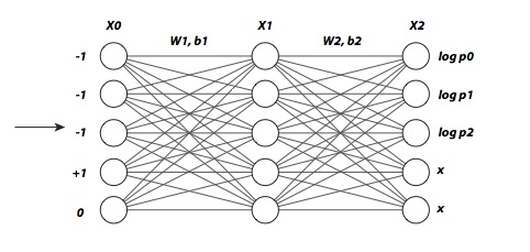
Note that in the output layer of the policy network shown, the first three values are labeled with log probabilities. These values correspond to the probabilities that we should next bomb each of these indices, respectively. We cannot re-bomb the fourth and fifth grid points, so although the network may output some values to these neurons, we’ll ignore them.

Before moving on, we note that the reason we use a neural network for our policy is to allow for efficient generalization: For games like Go that have a very large number of states, it is not feasible to collect data on every possible board position. This is exactly the context where ML algorithms excel — generalizing from past observations to make good predictions for new situations. In order to keep our focus on RL, we won’t review how ML algorithms work in this post (however, you can check out our archives section for relevant primers). Instead we simply note that — utilizing these tools — we can get good performance by training only on a representative subset of games — allowing us to avoid study of the full set, which can be much larger.

The rewards function

To train an RL algorithm, we must carry out an iterative game play / scoring process: We play games according to our current policy, selecting moves with frequencies proportional to the probabilities output by the network. If the actions taken resulted in good outcomes, we want to strengthen the probability of those actions going forward.

The rewards function is the tool we use to formally score our outcomes in past games — we will encourage our algorithm to try to maximize this quantity during game play. In effect, it is a hyper-parameter for the RL algorithm: many different functions could be used, each resulting in different learning characteristics. For our battleship program, we have used the function

\begin{align} \label{rewards} \tag{2} r(a;t_0) = \sum_{t \geq t_0} \left ( h(t) - \overline{h(t)} \right) (0.5)^{t-t0} \end{align}

Given a completed game log, this function looks at the action $a$ taken at time $t_0$ and returns a weighted sum of hit values $h(t)$ for this and all future steps in the game. Here, $h(t)$ is $1$ if we had a hit at step $t$ and is $0$ otherwise.

In arriving at (\ref{rewards}), we admit that we did not carry out a careful search over the set of all possible rewards functions. However, we have confirmed that this choice results in good game play, and it is well-motivated: In particular, we note that the weighting term $(0.5)^{t-t0}$ serves to strongly incentivize a hit on the current move (we get a reward of $1$ for a hit at $t_0$), but a hit at $(t_0 + 1)$ also rewards the action at $t_0$ — with value $0.5$. Similarly, a hit at $(t_0 + 2)$ rewards $0.25$, etc. This weighted look-ahead aspect of (\ref{rewards}) serves to encourage efficient exploration of the board: It forces the program to care about moves that will enable future hits. The other ingredient of note present in (\ref{rewards}) is the subtraction of $\overline{h(t)}$. This is the expected rewards that a random network would obtain. By pulling this out, we only reward our network if it is outperforming random choices — this results in a net speed-up of the learning process.

Stochastic gradient descent

In order to train our algorithm to maximize captured rewards during game play, we apply gradient descent. To carry this out, we imagine allowing our network parameters $\theta$ to vary at some particular step in the game. Averaging over all possible actions, the gradient of the expected rewards is then formally,

\begin{align} \nonumber \partial_{\theta} \langle r(a \vert s) \rangle &\equiv & \partial_{\theta} \int p(a \vert \theta, s) r(a \vert s) da \\ \nonumber &=& \int p(a \vert \theta, s) r(a \vert s) \partial_{\theta} \log \left ( p(a \vert \theta, s) \right) da \\ &\equiv & \langle r(a \vert s) \partial_{\theta} \log \left ( p(a \vert \theta, s) \right) \rangle. \tag{3} \label{formal_ev} \end{align}

Here, the $p(a)$ values are the action probability outputs of our network.

Unfortunately, we usually can’t evaluate the last line above. However, what we can do is approximate it using a sampled value: We simply play a game with our current network, then replace the expected value above by the reward actually captured on the $i$-th move,

\begin{align} \hat{g}_i = r(a_i) \nabla_{\theta} \log p(a_i \vert s_i, \theta). \tag{4} \label{estimator} \end{align}

Here, $a_i$ is the action that was taken, $r(a_i)$ is reward that was captured, and the derivative of the logarithm shown can be evaluated via back-propagation (aside for those experienced with neural networks: this is the derivative of the cross-entropy loss function that would apply if you treated the event like a supervised-learning training example — with the selected action $a_i$ taken as the label). The function $\hat{g}_i$ provides a noisy estimate of the desired gradient, but taking many steps will result in a “stochastic” gradient descent, on average pushing us towards correct rewards maximization.

Summary of the training process

In summary, then, RL training proceeds iteratively: To initialize an iterative step, we first play a game with our current policy network, selecting moves stochastically according to the network’s output. After the game is complete, we then score our outcome by evaluating the rewards captured on each move — for example, in the battleship game we use (\ref{rewards}). Once this is done, we then estimate the gradient of the rewards function using (\ref{estimator}). Finally, we update the network parameters, moving $\theta \to \theta + \alpha \sum \hat{g}_i$, with $\alpha$ a small step size parameter. To continue, we then play a new game with the updated network, etc.

To see that this process does, in fact, encourage actions that have resulted in good outcomes during training, note that (\ref{estimator}) is proportional to the rewards captured at the step $i$. Consequently, when we adjust our parameters in the direction of (\ref{estimator}), we will strongly encourage those actions that have resulted in large rewards outcomes. Further, those moves with negative rewards are actually suppressed. In this way, over time, the network will learn to examine the system and suggest those moves that will likely produce the best outcomes.

That’s it for the basics of deep, policy-gradient RL. We now turn to our python example, battleship.

Python code walkthrough — battleship RL

Load the needed packages.

import tensorflow as tf
import numpy as np
%matplotlib inline
import pylab

Define our network — a fully connected, three layer system. The code below is mostly tensorflow boilerplate that can be picked up by going through their first tutorials. The one unusual thing is that we have our learning rate in (26) set to the placeholder value (9). This will allow us to vary our step sizes with observed rewards captured below.

BOARD_SIZE = 10
SHIP_SIZE = 3

hidden_units = BOARD_SIZE
output_units = BOARD_SIZE

input_positions = tf.placeholder(tf.float32, shape=(1, BOARD_SIZE))
labels = tf.placeholder(tf.int64)
learning_rate = tf.placeholder(tf.float32, shape=[])
# Generate hidden layer
W1 = tf.Variable(tf.truncated_normal([BOARD_SIZE, hidden_units],
    stddev=0.1 / np.sqrt(float(BOARD_SIZE))))
b1 = tf.Variable(tf.zeros([1, hidden_units]))
h1 = tf.tanh(tf.matmul(input_positions, W1) + b1)
# Second layer -- linear classifier for action logits
W2 = tf.Variable(tf.truncated_normal([hidden_units, output_units],
    stddev=0.1 / np.sqrt(float(hidden_units))))
b2 = tf.Variable(tf.zeros([1, output_units]))
logits = tf.matmul(h1, W2) + b2
probabilities = tf.nn.softmax(logits)

init = tf.initialize_all_variables()
cross_entropy = tf.nn.sparse_softmax_cross_entropy_with_logits(
    logits, labels, name='xentropy')
train_step = tf.train.GradientDescentOptimizer(
learning_rate=learning_rate).minimize(cross_entropy)
# Start TF session
sess = tf.Session()
sess.run(init)

Next, we define a method that will allow us to play a game using our network. The TRAINING variable specifies whether or not to take the optimal moves or to select moves stochastically. Note that the method returns a set of logs that record the game proceedings. These are needed for training.

TRAINING = True
def play_game(training=TRAINING):
    """ Play game of battleship using network."""
    # Select random location for ship
    ship_left = np.random.randint(BOARD_SIZE - SHIP_SIZE + 1)
    ship_positions = set(range(ship_left, ship_left + SHIP_SIZE))
    # Initialize logs for game
    board_position_log = []
    action_log = []
    hit_log = []
    # Play through game
    current_board = [[-1 for i in range(BOARD_SIZE)]]
    while sum(hit_log) < SHIP_SIZE:
        board_position_log.append([[i for i in current_board[0]]])
        probs = sess.run([probabilities], feed_dict={input_positions:current_board})[0][0]
        probs = [p * (index not in action_log) for index, p in enumerate(probs)]
        probs = [p / sum(probs) for p in probs]
        if training == True:
            bomb_index = np.random.choice(BOARD_SIZE, p=probs)
        else:
            bomb_index = np.argmax(probs)
        # update board, logs
        hit_log.append(1 * (bomb_index in ship_positions))
        current_board[0][bomb_index] = 1 * (bomb_index in ship_positions)
        action_log.append(bomb_index)
    return board_position_log, action_log, hit_log

Our implementation of the rewards function (\ref{rewards}):

def rewards_calculator(hit_log, gamma=0.5):
    """ Discounted sum of future hits over trajectory"""
    hit_log_weighted = [(item -
    float(SHIP_SIZE - sum(hit_log[:index])) / float(BOARD_SIZE - index)) * (
        gamma ** index) for index, item in enumerate(hit_log)]
    return [((gamma) ** (-i)) * sum(hit_log_weighted[i:]) for i in range(len(hit_log))]

Finally, our training loop. Here, we iteratively play through many games, scoring after each game, then adjusting parameters — setting the placeholder learning rate equal to ALPHA times the rewards captured.

game_lengths = []
TRAINING = True # Boolean specifies training mode
ALPHA = 0.06 # step size

for game in range(10000):
    board_position_log, action_log, hit_log = play_game(training=TRAINING)
    game_lengths.append(len(action_log))
    rewards_log = rewards_calculator(hit_log)
    for reward, current_board, action in zip(rewards_log, board_position_log, action_log):
        # Take step along gradient
        if TRAINING:
            sess.run([train_step],
                feed_dict={input_positions:current_board, labels:[action], learning_rate:ALPHA * reward})

Running this last cell, we see that the training works! The following is an example trace from the play_game() method, with the variable TRAINING set to False. This illustrates an intelligent move selection process.

# Example game trace output
([[[-1, -1, -1, -1, -1, -1, -1, -1, -1, -1]],
[[-1, -1, 0, -1, -1, -1, -1, -1, -1, -1]],
[[-1, -1, 0, -1, -1, 0, -1, -1, -1, -1]],
[[-1, -1, 0, -1, -1, 0, 1, -1, -1, -1]],
[[-1, -1, 0, -1, -1, 0, 1, 1, -1, -1]]],
[2, 5, 6, 7, 8],
[0, 0, 1, 1, 1])

Here, the first five lines are the board encodings that the network was fed each step — using (\ref{input}). The second to last row presents the sequential grid selections that were chosen. Finally, the last row is the hit log. Notice that the first two moves nicely sample different regions of the board. After this, a hit was recorded at $6$. The algorithm then intelligently selects $7$ and $8$, which it can infer must be the final locations of the ship.

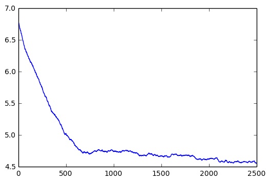
The plot below provides further characterization of the learning process. This shows the running average game length (steps required to fully bomb ship) versus training epoch. The program learns the basics quite quickly, then continues to gradually improve over time [2].

Summary

In this post, we have covered a variant of RL — namely, the policy-gradient, deep RL scheme. This is a method that typically defaults to the currently best-known strategy, but occasionally samples from other approaches, ultimately resulting in an iterative improvement in policy. The two main ingredients here are the policy network and the rewards function. Although network architecture design is usually the place where most of the thinking is involved in supervised learning, it is the rewards function that typically requires the most thought in the RL context. A good choice should be as local in time as possible, so as to facilitate training (distant forecast dependence will result in a slow learning process). However, the rewards function should also directly attack the ultimate end of the process (“winning” the game — encouragement of side quests that aren’t necessary can often occur if care is not taken). Balancing these two competing demands can be a challenge, and rewards function design is therefore something of an art form.

Our brief introduction here was intended only to illustrate the gist of how RL is carried out in practice. For further details, we can recommend two resources: the text book by Sutton and Barto [3] and a recent talk by John Schulman [4].

Footnotes and references

[1] Game rules: Battleship is a two-player game. Both players begin with a finite regular grid of positions — hidden from their opponent — and a set of “ships”. Each player receives the same quantity of each type of ship. At the start of the game, each player places the ships on their grid in whatever locations they like, subject to some constraints: A ship of length 2, say, must occupy two contiguous indices on the board, and no two ships can occupy the same grid location. Once placed, the ships are fixed in position for the remainder of the game. At this point, game play begins, with the goal being to sink the opponent ships. The locations of the enemy ships are initially unknown because we cannot see the opponent’s grid. To find the ships, one “bombs” indices on the enemy grid — with bombing occurs in turns. When an opponent index is bombed, the opponent must truthfully state whether or not a ship was located at the index bombed. Whoever succeeds in bombing all their opponent’s occupied indices first wins the game. Therefore, the problem reduces to finding the enemy ship indices as quickly as possible.

[2] One of my colleagues (HC) has suggested that the program likely begins to overfit at some point. However, the 1-d version of the game has so few possible ship locations that characterization of this effect via a training and test set split does not seem appropriate. However, this approach could work were we to move to higher dimensions and introduce multiple ships.

[3] Sutton and Barto, (2016). “Reinforcement Learning: An Introduction”. Text site, here.

[4] John Schulman, (2016). “Bay Area Deep Learning School”. Youtube recording of talk available here.

Jonathan Landy Jonathan grew up in the midwest and then went to school at Caltech and UCLA. Following this, he did two postdocs, one at UCSB and one at UC Berkeley. His academic research focused primarily on applications of statistical mechanics, but his professional passion has always been in the mastering, development, and practical application of slick math methods/tools. He currently works as a data-scientist at Stitch Fix.