In today’s post, we document our efforts at applying a gradient boosted trees model to forecast bike sharing demand — a problem posed in a recent Kagglecompetition. For those not familiar, Kaggle is a site where one can compete with other data scientists on various data challenges. Top scorers often win prize money, but the site more generally serves as a great place to grab interesting datasets to explore and play with. With the simple optimization steps discussed below, we managed to quickly move from the bottom 10% of the competition — our first-pass attempt’s score — to the top 10%: no sweat!
Our work here was inspired by a post by the people at Dato.com, who used the bike sharing competition as an opportunity to demonstrate their software. Here, we go through a similar, but more detailed discussion using the python package SKlearn.
Introduction
Bike sharing systems are gaining popularity around the world — there are over 500 different programs currently operating in various cities, and counting! These programs are generally funded through rider membership fees, or through pay-to-ride one time rental fees. Key to the convenience of these programs is the fact that riders who pick up a bicycle from one station can return the bicycle to any other in the network. These systems generate a great deal of data relating to various ride details, including travel time, departure location, arrival location, and so on. This data has the potential to be very useful for studying city mobility. The data we look at today comes from Washington D. C.’s Capital Bikeshare program. The goal of the Kaggle competition is to leverage the historical data provided in order to forecast future bike rental demand within the city.
As we detailed in an earlier post, boosting provides a general method for increasing a machine learning algorithm’s performance. Here, in order to model the Capital Bikeshare program’s demand curves, we’ll be applying a gradient boosted trees model (GBM). Simply put, GBM’s are constructed by iteratively fitting a series of simple trees to a training set, where each new tree attempts to fit the residuals, or errors, of the trees that came before it. With the addition of each new tree the training error is further reduced, typically asymptoting to a reasonably accurate model — but one must watch out for overfitting — see below!
Loading package and data
Below, we show the relevant commands needed to load all the packages and training/test data we will be using. We work with the package Pandas, whose DataFrame data structure enables quick and easy data loading and wrangling. We take advantage of this package immediately below, where in the last lines we use its parse_dates method to convert the first column of our provided data — which can be downloaded here — from string to datetime format.
import numpy as np
import matplotlib.pyplot as plt
import pandas as pd
import math

from sklearn import ensemble
from sklearn.cross_validation import train_test_split
from sklearn.metrics import mean_absolute_error
from sklearn.grid_search import GridSearchCV
from datetime import datetime

#Load Data with pandas, and parse the
#first column into datetime
train = pd.read_csv('train.csv', parse_dates=[0])
test = pd.read_csv('test.csv', parse_dates=[0])
The training data provided contains the following fields:
datetime - hourly date + timestamp season - 1 = spring, 2 = summer, 3 = fall, 4 = winter holiday - whether the day is considered a holiday workingday - whether the day is neither a weekend nor holiday weather:
- Clear, Few clouds, Partly cloudy, Partly cloudy
- Mist + Cloudy, Mist + Broken clouds, Mist + Few clouds, Mist
- Light Snow, Light Rain + Thunderstorm + Scattered clouds, Light Rain + Scattered clouds
- Heavy Rain + Ice Pallets + Thunderstorm + Mist, Snow + Fog
temp - temperature in Celsius atemp - “feels like” temperature in Celsius humidity - relative humidity windspeed - wind speed casual - number of non-registered user rentals initiated registered - number of registered user rentals initiated count - number of total rentals
The data provided spans two years. The training set contains the first 19 days of each month considered, while the test set data corresponds to the remaining days in each month.
Looking ahead, we anticipate that the year, month, day of week, and hour will serve as important features for characterizing the bike demand at any given moment. These features are easily extracted from the datetime formatted-values loaded above. In the following lines, we add these features to our DataFrames.
#Feature engineering
temp = pd.DatetimeIndex(train['datetime'])
train['year'] = temp.year
train['month'] = temp.month
train['hour'] = temp.hour
train['weekday'] = temp.weekday

temp = pd.DatetimeIndex(test['datetime'])
test['year'] = temp.year
test['month'] = temp.month
test['hour'] = temp.hour
test['weekday'] = temp.weekday

#Define features vector
features = ['season', 'holiday', 'workingday', 'weather',
'temp', 'atemp', 'humidity', 'windspeed', 'year',
'month', 'weekday', 'hour']
Evaluation metric
The evaluation metric that Kaggle uses to rank competing algorithms is the Root Mean Squared Logarithmic Error (RMSLE).
Here,
- \(n\) is the number of hours in the test set
- \(p_i\) is the predicted number of bikes rented in a given hour
- \(a_i\) is the actual rent count
- \(ln(x)\) is the natural logarithm
With ranking determined as above, our aim becomes to accurately guess the natural logarithm of bike demand at different times (actually demand count plus one, in order to avoid infinities associated with times where demand is nil). To facilitate this, we add the logarithm of the casual, registered, and total counts to our training DataFrame below.
#the evaluation metric is the RMSE in the log domain,
#so we should transform the target columns into log domain as well.
for col in ['casual', 'registered', 'count']:
  train['log-' + col] = train[col].apply(lambda x: np.log1p(x))
Notice that in the code above we use the \(log1p()\) function instead of the more familiar \(log(1+x)\). For large values of \(x\), these two functions are actually equivalent. However, at very small values of \(x\), the two can disagree. The source of the discrepancy is floating point error: For very small \(x\), python will send \(1+x \to 1\), which when supplied as an argument to \(log(1+x)\) will return \(log(1)=0\). The function \(log1p(x) \sim x\) in this limit. The difference is not very important when the result is being added to other numbers, but can be very important in a multiplicative operation. We use this function instead for this reason. The inverse of \(log(x+1)\) is \(e^{x} -1\) — an operation we will also need to make use of later, in order to return linear-scale demand values. We’ll use an analog of the \(log1p()\) function, numpy’s \(expm1()\) function, to carry out this inversion.
Model development
A first pass
The Gradient Boosting Machine (GBM) we will be using has some associated hyperparameters that will eventually need to be optimized. These include:
- n_estimators = the number of boosting stages, or trees, to use.
- max_depth = maximum depth of the individual regression trees.
- learning_rate = shrinks the contribution of each tree by the learning rate.
- in_samples_leaf = the minimum number of samples required to be at a leaf node
However, in order to get our feet wet, we’ll begin by just picking some ad hoc values for these parameters. The code below fits a GBM to the log-demand training data, and then converts predicted log-demand into the competition’s required format — in particular, the demand is output in linear scale.
clf = ensemble.GradientBoostingRegressor(
n_estimators=200, max_depth=3)
clf.fit(train[features], train['log-count'])
result = clf.predict(test[features])
result = np.expm1(result)

df=pd.DataFrame({'datetime':test['datetime'], 'count':result})
df.to_csv('results1.csv', index = False, columns=['datetime','count'])
In the last lines above, we have used the DataFrames to_csv() method in order to output results for competition submission. Example output is shown below. Without a hitch, we successfully submitted the results of this preliminary analysis to Kaggle. The only bad news was that our model scored in the bottom 10%. Fortunately, some simple optimizations that follow led to significant improvements in our standing.
| datetime | count |
|---|---|
| 2011-01-20 0:00:00 | 0 |
| 2011-01-20 0:01:00 | 0 |
| 2011-01-20 0:02:00 | 0 |
Hyperparameter tuning
We now turn to the challenge of tuning our GBM’s hyperparameters. In order to carry this out, we segmented our training data into a training set and a validation set. The validation set allowed us to check the accuracy of our model locally, without having to submit to Kaggle. This also helped us to avoid overfitting issues.
As mentioned earlier, the training data provided covers the first 19 days of each month. In segmenting this data, we opted to use days 17-19 for validation. We then used this validation set to optimize the model’s hyperparameters. As a first-pass at this, we again chose an ad hoc value for n_estimators, but optimized over the remaining degrees of freedom. The code follows, where we make use of GridSearchCV() to perform our parameter sweep.
#Split data into training and validation sets
temp = pd.DatetimeIndex(train['datetime'])
training = train[temp.day <= 16]
validation = train[temp.day > 16]

param_grid = {'learning_rate': [0.1, 0.05, 0.01],
              'max_depth': [10, 15, 20],
              'min_samples_leaf': [3, 5, 10, 20],
}

est = ensemble.GradientBoostingRegressor(n_estimators=500)
# this may take awhile
gs_cv = GridSearchCV(
est, param_grid, n_jobs=4).fit(
training[features], training['log-count'])

# best hyperparameter setting
gs_cv.best_params_

#Baseline error
error_count = mean_absolute_error(validation['log-count'], gs_cv.predict(validation[features]))

result = gs_cv.predict(test[features])
result = np.expm1(result)
df = pd.DataFrame({'datetime':test['datetime'], 'count':result})
df.to_csv('results2.csv', index = False, columns=['datetime','count'])
- Note: If you want to run n_jobs > 1 on a Windows machine, the script needs to be in an “if name == ‘main‘:” block. Otherwise the script will fail.
| day | Best Parms |
|---|---|
| 1 | learning_rate |
| 2 | max_depth |
| 2 | min_samples_leaf |
The optimized parameters are shown above. Submitting the resulting model to Kaggle, we found that we had moved from the bottom 10% of models to the top 20%! An awesome improvement, but we still have one final hyperparameter to optimize.
Tuning the number of estimators
In boosted models, training set performance will always improve as the number of estimators is increased. However, at large estimator number, overfitting can start to become an issue. Learning curves provide a method for optimization. These are constructed by plotting the error on both the training and validation sets as a function of the number of estimators used. The code below generates such a curve for our model.
error_train=[]
error_validation=[]
for k in range(10, 501, 10):
  clf = ensemble.GradientBoostingRegressor(
  n_estimators=k, learning_rate = .05, max_depth = 10,
  min_samples_leaf = 20)

  clf.fit(training[features], training['log-count'])
  result = clf.predict(training[features])
  error_train.append(
  mean_absolute_error(result, training['log-count']))

  result = clf.predict(validation[features])
  error_validation.append(
  mean_absolute_error(result, validation['log-count']))

#Plot the data
x=range(10,501, 10)
plt.style.use('ggplot')
plt.plot(x, error_train, 'k')
plt.plot(x, error_validation, 'b')
plt.xlabel('Number of Estimators', fontsize=18)
plt.ylabel('Error', fontsize=18)
plt.legend(['Train', 'Validation'], fontsize=18)
plt.title('Error vs. Number of Estimators', fontsize=20)
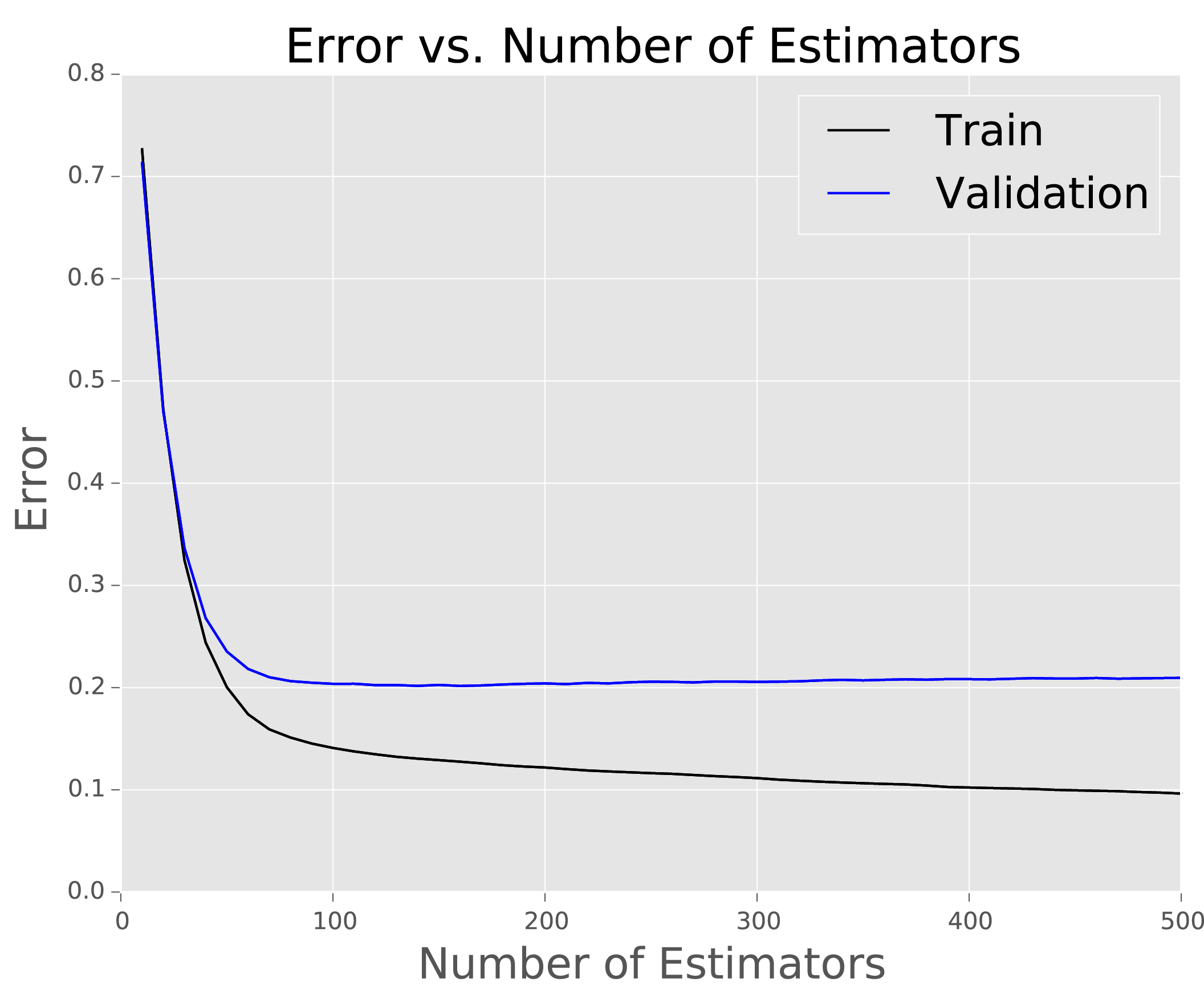
Notice in the plot that by the time the number estimators in our GBM reaches about 80, the error of our model as applied to the validation set starts to slowly increase, though the error on the training set continues to decrease steadily. The diagnosis is that the model begins to overfit at this point. Moving forward, we will set n_estimators to 80, rather than 500, the value we were using above. Reducing the number of estimators reduced the calculated error and moved us to a higher position on the leaderboard.
Separate models for registered and casual users
Reviewing the data, we see that we have info regarding two types of riders: casual and registered riders. It is plausible that each group’s behavior differs, and that we might be able to improve our performance by modeling each separately. Below, we carry this out, and then also merge the two group’s predicted values to obtain a net predicted demand. We also repeat the hyperparameter sweep steps covered above — this returned similar values. Resubmitting the resulting model, we found we had increased our standing in the competition by a few percent.
def merge_predict(model1, model2, test_data):
  # Combine the predictions of two separately trained models.
  # The input models are in the log domain and returns the predictions
  # in original domain.
  p1 = np.expm1(model1.predict(test_data))
  p2 = np.expm1(model2.predict(test_data))
  p_total = (p1+p2)
  return(p_total)
est_casual = ensemble.GradientBoostingRegressor(n_estimators=80, learning_rate = .05)
est_registered = ensemble.GradientBoostingRegressor(n_estimators=80, learning_rate = .05)
param_grid2 = {'max_depth': [10, 15, 20],
               '_samples_leaf': [3, 5, 10, 20],
}

gs_casual = GridSearchCV(est_casual, param_grid2, n_jobs=4).fit(training[features], training['log-casual'])
gs_registered = GridSearchCV(est_registered, param_grid2, n_jobs=4).fit(training[features], training['log-registered'])

result3 = merge_predict(gs_casual, gs_registered, test[features])
df = pd.DataFrame({'datetime':test['datetime'], 'count':result3})
df.to_csv('results3.csv', index = False, columns=['datetime','count'])
The last step is to submit a final set of model predictions, this time training on the full labeled dataset provided. With these simple steps, we ended up in the top 11% on the competition’s leaderboard with a rank of 280/2467!

<pre>
est_casual = ensemble.GradientBoostingRegressor(
n_estimators=80, learning_rate = .05, max_depth = 10,min_samples_leaf = 20)
est_registered = ensemble.GradientBoostingRegressor(
n_estimators=80, learning_rate = .05, max_depth = 10,min_samples_leaf = 20)

est_casual.fit(train[features].values, train['log-casual'].values)
est_registered.fit(train[features].values, train['log-registered'].values)
result4 = merge_predict(est_casual, est_registered, test[features])

df=pd.DataFrame({'datetime':test['datetime'], 'count':result4})
df.to_csv('results4.csv', index = False, columns=['datetime','count'])
DISCUSSION
By iteratively tuning a GBM, we were able to quickly climb the leaderboard for this particular Kaggle competition. With further feature extraction work, we believe further improvements could readily be made. However, our goal here was only to practice our rapid development skills, so we won’t be spending much time on further fine-tuning. At any rate, our results have convinced us that simple boosted models can often provide excellent results.
![]() Open GitHub Repo
Open GitHub Repo
Note: With this post, we have begun to post our python scripts and data at GitHub. Clicking on the icon at left will take you to our repository. Feel free to stop by and take a look!
 Damien is a highly experienced researcher with a background in clinical and applied research. Like JSL, he got his PhD at UCLA. He has many years of experience working with imaging, and has a particularly strong background in image segmentation, registration, detection, data analysis, and more recently machine learning. He now works as a data-scientist at Square in San Francisco.