Here, we characterize the data compression benefits of projection onto a subset of the eigenvectors of our traffic system’s covariance matrix. We address this compression from two different perspectives: First, we consider the partial traces of the covariance matrix, and second we present visual comparisons of the actual vs. projected traffic plots.
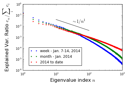
Partial traces: From the footnote to our last post, we have \(\text{Tr}(H^{-1}) \equiv \sum_i e_i = \sum_a \left (\delta v_a \right)^2\). That is, the trace of the covariance matrix tells us the net variance in our traffic system’s speed, summed over all loops. More generally\(^1\), the fraction of system variance contained within some subset of the modes is given by the eigenvalue sum over these modes, all divided by \(\text{Tr}(H^{-1})\). The eigenvalues thus provide us with a simple method for quantifying the significance of any particular mode. At right, is a log-log-plot of the fractional-variance-captured for each mode, ordered from largest to smallest (we also include analogous plots for the covariance matrix associated with just one week and one month\(^2\)) As shown, the eigenvalues decay like one over eigenvalue index at first, but eventually begin to decay much more quickly. Only 5 modes are needed to capture 50% of the variance; 25 for 65%; 793 for 95%.
Visualizations: The above discussion suggests that the basic essence of a given set of traffic conditions is determined by only the first few modes, but that a large number might be needed to get correct all details. We tested this conclusion by visually inspecting plots of projected traffic conditions (again, for Jan 15, at 5:30 pm), and comparing across number of modes retained. The results are striking: upon projecting the 2,000+ original features to only 25, minimal error appears to be introduced. Further, the error that does occur tends to be highly localized to the particularly slow regions, where projected speeds are overestimates (e.g., the traffic jams east/south-bound out of Oakland). Increasing the mode count to 100 or greater, these problem spots are quickly ameliorated, and the error is no longer systematic in slow regions (see insets).
Conclusions: The data provided by the PEMS system is highly redundant — as anticipated — in the sense that traffic conditions can be determined from far fewer measurements than it provides. If other states wanted to replicate this system, they could probably get away with reducing the number of measures by at least one order of magnitude per mile of highway. For our part, we intend to project our data onto the top 10% of the modes, or fewer: We anticipate that this will provide minimal loss, but substantial speedups.
[1] Partial eigenvalue sums, physics perspective: Consider suppressing all modes that you don’t want to include in a projection. This can be done by setting the energies of these modes to \(\infty\), which will result in their corresponding \(H^{-1}\) eigenvalues going to zero. When this altered system is thermally driven, its variance will again be given its covariance trace. This altered system trace is precisely equal to the retained mode partial sum of the original matrix.
[2] Sampling time dependence of covariance matrix: The first figure above shows the mode variance ratio for the first 1000 principal components over three time scales: 1 week, 1 month, and 2014 year to date (~9.5 months). Notice that the plots become more shallow given a longer sampling period. This is because the larger data sets exhibit a more diverse class of fluctuations, and more modes are needed to capture these.
 Dustin got a B.S in Engineering Physics from the Colorado School of Mines (Golden, CO) before moving to UC Santa Barbara for graduate school. There he became interested in Soft Condensed Matter Physics and Polymer Physics, studying the interaction between single DNA molecules and salt ions. After a brief postdoc at UC San Diego studying the physics of bacterial growth, Dustin decided to move into the data science business for good - he is now a Quantitative Analyst at Google in Mountain View.