Gaussian Processes

We review the math and code needed to fit a Gaussian Process (GP) regressor to data. We conclude with a demo of a popular application, fast function minimization through GP-guided search. The gif below illustrates this approach in action — the red points are samples from the hidden red curve. Using these samples, we attempt to leverage GPs to find the curve’s minimum as fast as possible.

Appendices contain quick reviews on (i) the GP regressor posterior derivation, (ii) SKLearn’s GP implementation, and (iii) GP classifiers.

Introduction

Gaussian Processes (GPs) provide a tool for treating the following general problem: A function \(f(x)\) is sampled at \(n\) points, resulting in a set of noisy\(^1\) function measurements, \(\{f(x_i) = y_i \pm \sigma_i, i = 1, \ldots, n\}\). Given these available samples, can we estimate the probability that \(f = \hat{f}\), where \(\hat{f}\) is some candidate function?

To decompose and isolate the ambiguity associated with the above challenge, we begin by applying Bayes’s rule,

\begin{eqnarray} \label{Bayes} \tag{1} p(\hat{f} \vert \{y\}) = \frac{p(\{y\} \vert \hat{f} ) p(\hat{f})}{p(\{y\}) }. \end{eqnarray}

The quantity at left above is shorthand for the probability we seek — the probability that \(f = \hat{f}\), given our knowledge of the sampled function values \(\{y\}\). To evaluate this, one can define and then evaluate the quantities at right. Defining the first in the numerator requires some assumption about the source of error in our measurement process. The second function in the numerator is the prior — it is here where the greatest assumptions must be taken. For example, we’ll see below that the prior effectively dictates the probability of a given smoothness for the \(f\) function in question.

In the GP approach, both quantities in the numerator at right above are taken to be multivariate Normals / Gaussians. The specific parameters of this Gaussian can be selected to ensure that the resulting fit is good — but the Normality requirement is essential for the mathematics to work out. Taking this approach, we can write down the posterior analytically, which then allows for some useful applications. For example, we used this approach to obtain the curves shown in the top figure of this post — these were obtained through random sampling from the posterior of a fitted GP, pinned to equal measured values at the two pinched points shown. Posterior samples are useful for visualization and also for taking Monte Carlo averages.

In this post, we (i) review the math needed to calculate the posterior above, (ii) discuss numerical evaluations and fit some example data using GPs, and (iii) review how a fitted GP can help to quickly minimize a cost function — eg a machine learning cross-validation score. Appendices cover the derivation of the GP regressor posterior, SKLearn’s GP implementation, and GP Classifiers.

Our minimal python class SimpleGP used below is available on our GitHub, here.

Note: To understand the mathematical details covered in this post, one should be familiar with multivariate normal distributions — these are reviewed in our prior post, here. These details can be skipped by those primarily interested in applications.

Analytic evaluation of the posterior

To evaluate the left side of (\ref{Bayes}), we will evaluate the right. Only the terms in the numerator need to be considered, because the denominator does not depend on \(\hat{f}\). This means that the denominator must equate to a normalization factor, common to all candidate functions. In this section, we will first write down the assumed forms for the two terms in the numerator and then consider the posterior that results.

The first assumption that we will make is that if the true function is \(\hat{f}\), then our \(y\)-measurements are independent and Gaussian-distributed about \(\hat{f}(x)\). This assumption implies that the first term on the right of (\ref{Bayes}) is

\begin{eqnarray} \tag{2} \label{prob} p(\{y\} \vert \hat{f} ) \equiv \prod_{i=1}^n \frac{1}{\sqrt{2 \pi \sigma_i^2}} \exp \left ( - \frac{(y_i - \hat{f}(x_i) )^2}{2 \sigma_i^2} \right). \end{eqnarray}

The \(y_i\) above are the actual measurements made at our sample points, and the \(\sigma_i^2\) are their variance uncertainties.

The second thing we must do is assume a form for \(p(\hat{f})\), our prior. We restrict attention to a set of points \(\{x_i: i = 1, \ldots, N\}\), where the first \(n\) points are the points that have been sampled, and the remaining \((N-n)\) are test points at other locations — points where we would like to estimate the joint statistics\(^2\) of \(f\). To progress, we simply assume a multi-variate Normal distribution for \(f\) at these points, governed by a covariance matrix \(\Sigma\). This gives

\begin{eqnarray} \label{prior} \tag{3} &&p(f(x_1), \ldots, f(x_N) ) \sim \ && \frac{1}{\sqrt{ (2 \pi)^{N} \vert \Sigma \vert }} \exp \left ( - \frac{1}{2} \sum_{ij=1}^N f_i \Sigma^{-1}_{ij} f_j \right). \end{eqnarray}

Here, we have introduced the shorthand, \(f_i \equiv f(x_i)\). Notice that we have implicitly assumed that the mean of our normal distribution is zero above. This is done for simplicity: If a non-zero mean is appropriate, this can be added in to the analysis, or subtracted from the underlying \(f\) to obtain a new one with zero mean.

The particular form of \(\Sigma\) is where all of the modeler’s insight and ingenuity must be placed when working with GPs. Researchers who know their topic very well can assert well-motivated, complex priors — often taking the form of a sum of terms, each capturing some physically-relevant contribution to the statistics of their problem at hand. In this post, we’ll assume the simple form

\begin{eqnarray} \tag{4} \label{covariance} \Sigma_{ij} \equiv \sigma^2 \exp \left( - \frac{(x_i - x_j)^2}{2 l^2}\right). \end{eqnarray}

Notice that with this assumed form, if \(x_i\) and \(x_j\) are close together, the exponential will be nearly equal to one. This ensures that nearby points are highly correlated, forcing all high-probability functions to be smooth. The rate at which (\ref{covariance}) dies down as two test points move away from each another is controlled by the length-scale parameter \(l.\) If this is large (small), the curve will be smooth over a long (short) distance. We illustrate these points in the next section, and also explain how an appropriate length scale can be inferred from the sample data at hand in the section after that.

Now, if we combine (\ref{prob}) and (\ref{prior}) and plug this into (\ref{Bayes}), we obtain an expression for the posterior, \(p(f \vert \{y\})\). This function is an exponential whose argument is a quadratic in the \(f_i\). In other words, like the prior, the posterior is a multi-variate normal. With a little work, one can derive explicit expressions for the mean and covariance of this distribution: Using block notation, with \(0\) corresponding to the sample points and \(1\) to the test points, the marginal distribution at the test points is

\begin{eqnarray} \tag{5} \label{posterior} && p(\textbf{f}_1 \vert \{y\}) =\ && N\left ( \Sigma_{10} \frac{1}{\sigma^2 I_{00} + \Sigma_{00}} \cdot \textbf{y}, \Sigma_{11} - \Sigma_{10} \frac{1}{\sigma^2 I_{00} + \Sigma_{00}} \Sigma_{01} \right). \end{eqnarray}

Here,

\begin{eqnarray} \tag{6} \label{sigma_mat} \sigma^2 I_{00} \equiv \left( \begin{array}{cccc} \sigma_1^2 & 0 & \ldots &0 \\ 0 & \sigma_2^2 & \ldots &0 \\ \ldots & & & \\ 0 & 0 & \ldots & \sigma_n^2 \end{array} \right), \end{eqnarray}

and \(\textbf{y}\) is the length-\(n\) vector of measurements,

\begin{eqnarray}\tag{7} \label{y_vec} \textbf{y}^T \equiv (y_1, \ldots, y_n). \end{eqnarray}

Equation (\ref{posterior}) is one of the main results for Gaussian Process regressors — this result is all one needs to evaluate the posterior. Notice that the mean at all points is linear in the sampled values \(\textbf{y}\) and that the variance at each point is reduced near the measured values. Those interested in a careful derivation of this result can consult our appendix — we actually provide two derivations there. However, in the remainder of the body of the post, we will simply explore applications of this formula.

Numerical evaluations of the posterior

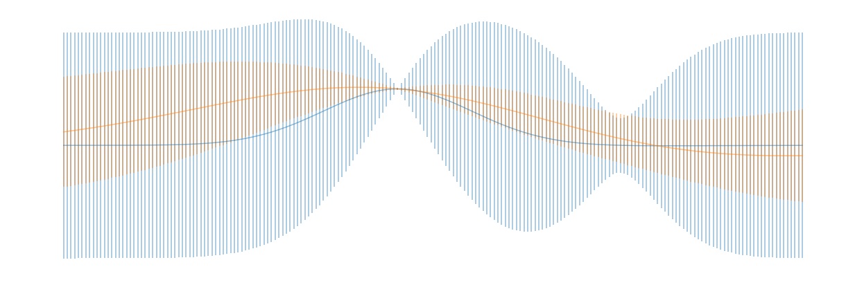
In this section, we will demonstrate how two typical applications of (\ref{posterior}) can be carried out: (i) Evaluation of the mean and standard deviation of the posterior distribution at a test point \(x\), and (ii) Sampling functions \(\hat{f}\) directly from the posterior. The former is useful in that it can be used to obtain confidence intervals for \(f\) at all locations, and the latter is useful both for visualization and also for obtaining general Monte Carlo averages over the posterior. Both concepts are illustrated in the header image for this post: In this picture, we fit a GP to a one-d function that had been measured at two locations. The blue shaded region represents a one-sigma confidence interval for the function value at each location, and the colored curves are posterior samples.

The code for our SimpleGP fitter class is available on our GitHub. We’ll explain a bit how this works below, but those interested in the details should examine the code — it’s a short script and should be largely self-explanatory.

Intervals

The code snippet below initializes our SimpleGP class, defines some sample locations, values, and uncertainties, then evaluates the mean and standard deviation of the posterior at a set of test points. Briefly, this carried out as follows: The fit method evaluates the inverse matrix \(\left [ \sigma^2 I_{00} + \Sigma_{00} \right]^{-1}\) that appears in (\ref{posterior}) and saves the result for later use — this allows us to avoid reevaluation of this inverse at each test point. Next, (\ref{posterior}) is evaluated once for each test point through the call to the interval method.

# Initialize fitter -- set covariance parameters
WIDTH_SCALE = 1.0
LENGTH_SCALE = 1.0
model = SimpleGP(WIDTH_SCALE, LENGTH_SCALE, noise=0)

# Insert observed sample data here, fit
sample_x = [-0.5, 2.5]
sample_y = [.5, 0]
sample_s = [0.01, 0.25]
model.fit(sample_x, sample_y, sample_s)

# Get the mean and std at each point in x_test
test_x = np.arange(-5, 5, .05)
means, stds = model.interval(test_x)

In the above, WIDTH_SCALE and LENGTH_SCALE are needed to specify the covariance matrix (\ref{covariance}). The former corresponds to \(\sigma\) and the latter to \(l\) in that equation. Increasing WIDTH_SCALE corresponds to asserting less certainty as to the magnitude of unknown function and increasing LENGTH_SCALE corresponds to increasing how smooth we expect the function to be. The figure below illustrates these points: Here, the blue intervals were obtained by setting WIDTH_SCALE = LENGTH_SCALE = 1 and the orange intervals were obtained by setting WIDTH_SCALE = 0.5 and LENGTH_SCALE = 2. The result is that the orange posterior estimate is tighter and smoother than the blue posterior. In both plots, the solid curve is a plot of the mean of the posterior distribution, and the vertical bars are one sigma confidence intervals.

Posterior samples

To sample actual functions from the posterior, we will simply evaluate the mean and covariance matrix in (\ref{posterior}) again, this time passing in the multiple test point locations at which we would like to know the resulting sampled functions. Once we have the mean and covariance matrix of the posterior at these test points, we can pull samples from (\ref{posterior}) using an external library for multivariate normal sampling — for this purpose, we used the python package numpy. The last step in the code snippet below carries out these steps.

# Insert observed sample data here.
sample_x = [-1.5, -0.5, 0.7, 1.4, 2.5, 3.0]
sample_y = [1, 2, 2, .5, 0, 0.5]
sample_s = [0.01, 0.25, 0.5, 0.01, 0.3, 0.01]

# Initialize fitter -- set covariance parameters
WIDTH_SCALE = 1.0
LENGTH_SCALE = 1.0
model = SimpleGP(WIDTH_SCALE, LENGTH_SCALE, noise=0)
model.fit(sample_x, sample_y, sample_s)

# Get the mean and std at each point in test_x
test_x = np.arange(-5, 5, .05)
means, stds = model.interval(test_x)

# Sample here
SAMPLES = 10
samples = model.sample(test_x, SAMPLES)

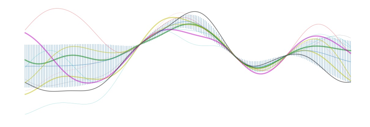
Notice that in lines 2-4 here, we’ve added in a few additional function sample locations (for fun). The resulting intervals and posterior samples are shown in the figure below. Notice that near the sampled points, the posterior is fairly well localized. However, on the left side of the plot, the posterior approaches the prior once we have moved a distance \(\geq 1\), the length scale chosen for the covariance matrix (\ref{covariance}).

Selecting the covariance hyper-parameters

In the above, we demonstrated that the length scale of our covariance form dramatically affects the posterior — the shape of the intervals and also of the samples from the posterior. Appropriately setting these parameters is a general problem that can make working with GPs a challenge. Here, we describe two methods that can be used to intelligently set such hyper-parameters, given some sampled data.

Cross-validation

A standard method for setting hyper-parameters is to make use of a cross-validation scheme. This entails splitting the available sample data into a training set and a test set. One fits the GP to the training set using one set of hyper-parameters, then evaluates the accuracy of the model on the held out test set. One then repeats this process across many hyper-parameter choices, and selects that set which resulted in the best test set performance.

Marginal Likelihood Maximization

Often, one is interested in applying GPs in limits where evaluation of samples is expensive. This means that one often works with GPs in limits where only a small number of samples are available. In cases like this, the optimal hyper-parameters can vary quickly as the number of training points is increased. This means that the optimal selections obtained from a cross-validation schema may be far from the optimal set that applies when one trains on the full sample set\(^3\).

An alternative general approach for setting the hyper-parameters is to maximize the marginal likelihood. That is, we try to maximize the likelihood of seeing the samples we have seen — optimizing over the choice of available hyper-parameters. Formally, the marginal likelihood is evaluated by integrating out the unknown \(\hat{f}^4\),

\begin{eqnarray} \tag{8} p(\{y\} \vert \Sigma) \equiv \int p(\{y\} \vert f) p(f \vert \Sigma) df. \end{eqnarray}

Carrying out the integral directly can be done just as we have evaluated the posterior distribution in our appendix. However, a faster method is to note that after integrating out the \(f\), the \(y\) values must be normally distributed as

\begin{eqnarray}\tag{9} p(\{y\} \vert \Sigma) \sim N(0, \Sigma + \sigma^2 I_{00}), \end{eqnarray}

where \(\sigma^2 I_{00}\) is defined as in (\ref{sigma_mat}). This gives

\begin{eqnarray} \tag{10} \label{marginallikelihood} \log p(\{y\}) \sim - \log \vert \Sigma + \sigma^2 I_{00} \vert - \textbf{y} \cdot ( \Sigma + \sigma^2 I_{00} )^{-1} \cdot \textbf{y}. \end{eqnarray}

The two terms above compete: The second term is reduced by finding the covariance matrix that maximizes the exponent. Maximizing this alone would tend to result in an overfitting of the data. However, this term is counteracted by the first, which is the normalization for a Gaussian integral. This term becomes larger given short decay lengths and low diagonal variances. It acts as regularization term that suppresses overly complex fits.

In practice, to maximize (\ref{marginallikelihood}), one typically makes use of gradient descent, using analytical expressions for the gradient. This is the approach taken by SKLearn. Being able to optimize the hyper-parameters of a GP is one of this model’s virtures. Unfortunately, (\ref{marginallikelihood}) is not guaranteed to be convex and multiple local minima often exist. To obtain a good minimum, one can attempt to initialize at some well-motivated point. Alternatively, one can reinitialize the gradient descent repeatedly at random points, finally selecting the best option at the end.

Function minimum search and machine learning

We’re now ready to introduce one of the popular application of GPs: fast, guided function minimum search. In this problem, one is able to iteratively obtain noisy samples of a function, and the aim is to identify as quickly as possible the global minimum of the function. Gradient descent could be applied in cases like this, but this approach generally requires repeated sampling if the function is not convex. To reduce the number of steps / samples required, one can attempt to apply a more general, explore-exploit type strategy — one balancing the desire to optimize about the current best known minimum with the goal of seeking out new local minima that are potentially even better. GP posteriors provide a natural starting point for developing such strategies.

The idea behind the GP-guided search approach is to develop a score function on top of the GP posterior. This score function should be chosen to encode some opinion of the value of searching a given point — preferably one that takes an explore-exploit flavor. Once each point is scored, the point with the largest (or smallest, as appropriate) score is sampled. The process is then repeated iteratively until one is satisfied. Many score functions are possible. We discuss four possible choices below, then give an example.

Gaussian Lower Confidence Bound (GLCB). The GLCB scores each point \(x\) as
\begin{eqnarray}\tag{11} s_{\kappa}(x) = \mu(x) - \kappa \sigma(x). \end{eqnarray}
Here, \(\mu\) and \(\sigma\) are the GP posterior estimates for the mean and standard deviation for the function at \(x\) and \(\kappa\) is a control parameter. Notice that the first \(\mu(x)\) term encourages exploitation around the best known local minimum. Similarly, the second \(\kappa \sigma\) term encourages exploration — search at points where the GP is currently most unsure of the true function value.
Gaussian Probability of Improvement (GPI). If the smallest value seen so far is \(y\), we can score each point using the probability that the true function value at that point is less than \(y\). That is, we can write
\begin{eqnarray}\tag{12} s(x) = \frac{1}{\sqrt{2 \pi \sigma^2}} \int_{-\infty}^y e^{-(v - \mu)^2 / (2 \sigma^2)} dv. \end{eqnarray}
Gaussian Expected Improvement (EI). A popular variant of the above is the so-called expected improvement. This is defined as
\begin{eqnarray} \tag{13} s(x) = \frac{1}{\sqrt{2 \pi \sigma^2}} \int_{-\infty}^y e^{-(v - \mu)^2 / (2 \sigma^2)} (y - v) dv. \end{eqnarray}
This score function tends to encourage more exploration than the probability of improvement, since it values uncertainty more highly.
Probability is minimum. A final score function of interest is simply the probability that the point in question is the minimum. One way to obtain this score is to sample from the posterior many times. For each sample, we mark its global minimum, then take a majority vote for where to sample next.

The gif at the top of this page (copied below) illustrates an actual GP-guided search, carried out in python using the package skopt\(^5\). The red curve at left is the (hidden) curve \(f\) whose global minimum is being sought. The red points are the samples that have been obtained so far, and the green shaded curve is the GP posterior confidence interval for each point — this gradually improves as more samples are obtained. At right is the Expected Improvement (EI) score function at each point that results from analysis on top of the GP posterior — the score function used to guide search in this example. The process is initialized with five random samples, followed by guided search. Notice that as the process evolves, the first few samples focus on exploitation of known local minima. However, after a handful of iterations, the diminishing returns of continuing to sample these locations loses out to the desire to explore the middle points — where the actual global minimum sits and is found.

Discussion

In this post we’ve overviewed much of the math of GPs: The math needed to get to the posterior, how to sample from the posterior, and finally how to make practical use of the posterior.

In principle, GPs represent a powerful tool that can be used to fit any function. In practice, the challenge in wielding this tool seems to sit mainly with selection of appropriate hyper-parameters — the search for appropriate parameters often gets stuck in local minima, causing fits to go off the rails. Nevertheless, when done correctly, application of GPs can provide some valuable performance gains — and they are always fun to visualize.

Some additional topics relating to GPs are contained in our appendices. For those interested in even more detail, we can recommend the free online text by Rasmussen and Williams\(^6\).

Appendix A: Derivation of posterior

In this appendix, we present two methods to derive the posterior (\ref{posterior}).

Method 1

We will begin by completing the square. Combining (\ref{prob}) and (\ref{prior}), a little algebra gives

\begin{align} \tag{A1} \label{square_complete} p(f_1, \ldots, f_N \vert \{y\}) &\sim \exp \left (-\sum_{i=1}^n \frac{(y_i - f_i)^2}{2 \sigma^2_i} - \frac{1}{2} \sum_{ij=1}^N f_i \Sigma^{-1}_{ij} f_j \right) \\ &\sim N\left ( \frac{1}{\Sigma^{-1} + \frac{1}{\sigma^2} I } \cdot \frac{1}{\sigma^2} I \cdot \textbf{y}, \frac{1}{\Sigma^{-1} + \frac{1}{\sigma^2} I } \right). \end{align}

Here, \(\frac{1}{\sigma^2} I\) is defined as in (\ref{sigma_mat}), but has zeros in all rows outside of the sample set. To obtain the expression (\ref{posterior}), we must identify the block structure of the inverse matrix that appears above.

To start, we write

\begin{align} \tag{A2} \label{matrix_to_invert} \frac{1}{\Sigma^{-1} + \frac{1}{\sigma^2}I } &= \Sigma \frac{1}{I + \frac{1}{\sigma^2}I \Sigma} \\ &= \Sigma \left( \begin{matrix} I_{00} + \frac{1}{\sigma^2}I_{00} \Sigma_{00} & \frac{1}{\sigma^2}I_{00} \Sigma_{01}\\ 0 & I_{11} \end{matrix} \right)^{-1}, \end{align}

where we are using block notation. To evaluate the inverse that appears above, we will make use of the block matrix inversion formula,

\begin{align} &\left( \begin{matrix} A & B\\ C & D \end{matrix} \right)^{-1} = \\ &\left( \begin{matrix} (A - B D^{-1} C)^{-1} & - (A - B D^{-1} C)^{-1} B D^{-1} \\ -D^{-1} C (A - B D^{-1} C)^{-1} & D^{-1} + D^{-1} C (A - B D^{-1} C) B D^{-1} \end{matrix} \right). \end{align}

The matrix (\ref{matrix_to_invert}) has blocks \(C = 0\) and \(D=I\), which simplifies the above significantly. Plugging in, we obtain

\begin{align} \label{shifted_cov} \tag{A3} \frac{1}{\Sigma^{-1} + \frac{1}{\sigma^2}I } = \Sigma \left( \begin{matrix} \frac{1}{I_{00} + \frac{1}{\sigma^2}I \Sigma_{00}} & - \frac{1}{I_{00} + \frac{1}{\sigma^2}I \Sigma_{00}} \Sigma_{01}\\ 0 & I_{11} \end{matrix} \right) \end{align}

With this result and (\ref{square_complete}), we can read off the mean of the test set as

\begin{align} \tag{A4} \label{mean_test} & \left [ [ \Sigma^{-1} + \frac{1}{\sigma^2} I_{00} ]^{-1} \cdot \frac{1}{\sigma^2} I_{00} \cdot \textbf{y} \right ]_1 \\ &= \Sigma_{10} \frac{1}{I_{00} + \frac{1}{\sigma^2}I_{00} \Sigma_{00}} \frac{1}{\sigma^2} I_{00} \cdot \textbf{y} \\ &= \Sigma_{10} \frac{1}{\sigma^2 I_{00} + \Sigma_{00}} \cdot \textbf{y}, \end{align}

where we have multiplied the numerator and denominator by the inverse of \(\frac{1}{\sigma^2}I_{00}\) in the second line. Similarly, the covariance of the test set is given by the lower right block of (\ref{shifted_cov}). This is,

\begin{align}\tag{A5} \label{covariance_test} \Sigma_{11} - \Sigma_{10} \cdot \frac{1}{\sigma^2 I_{00} + \Sigma_{00}} \cdot \Sigma_{01}. \end{align}

The results (\ref{mean_test}) and (\ref{covariance_test}) give (\ref{posterior}).

Method 2

In this second method, we consider the joint distribution of a set of test points \(\textbf{f}_1\) and the set of observed samples \(\textbf{f}_0\). Again, we assume that the function density has mean zero. The joint probability density for the two is then

\begin{align}\tag{A6} p(\textbf{f}_0, \textbf{f}_1) \sim N \left ( \left ( \begin{matrix} 0 \\ 0 \end{matrix} \right), \left ( \begin{matrix}{cc} \Sigma_{0,0} & \Sigma_{0,1} \\ \Sigma_{1,0} & \Sigma_{11} \end{matrix} \right ) \right ) \end{align}

Now, we use the result

\begin{align} \tag{A7} p( \textbf{f}_1 \vert \textbf{f}_0) &=& \frac{p( \textbf{f}_0, \textbf{f}_1)}{p( \textbf{f}_0)}. \end{align}

The last two expressions are all that are needed to derive (\ref{posterior}). The main challenge involves completing the square, and this can be done with the block matrix inversion formula, as in the previous derivation.

Appendix B: SKLearn implementation and other kernels

SKLearn provides contains the GaussianProcessRegressor class. This allows one to carry out fits and sampling in any dimension — i.e., it is more general than our minimal class in that it can fit feature vectors in more than one dimension. In addition, the fit method of the SKLearn class attempts to find an optimal set of hyper-parameters for a given set of data. This is done through maximization of the marginal likelihood, as described above. Here, we provide some basic notes on this class and the built in kernels that one can use to define the covariance matrix \(\Sigma\) in (\ref{prior}). We also include a simple code snippet illustrating calls.

Pre-defined Kernels

Radial-basis function (RBF): This is the default — equivalent to our (\ref{covariance}). The RBF is characterized by a scale parameter, \(l\). In more than one dimension, this can be a vector, allowing for anisotropic correlation lengths.
White kernel : The White Kernel is used for noise estimation — docs suggest useful for estimating the global noise level, but not pointwise.
Matern: This is a generalized exponential decay, where the exponents is a powerlaw in separation distance. Special limits include the RBF and also an absolute distance exponential decay. Some special parameter choices allow for existence of single or double derivatives.
Rational quadratic: This is \((1 + (d / l)^2)^{\alpha}\).
Exp-Sine-Squared: This allows one to model periodic functions. This is just like the RBF, but the distance that gets plugged in is the sine of the actual distance. A periodicity parameter exists, as well as a “variance” — the scale of the Gaussian suppression.
Dot product kernel : This takes form \(1 + x_i \cdot x_j\). It’s not stationary, in the sense that the result changes if a constant translation is added in. They state that you get this result from linear regression analysis if you place \(N(0,1)\) priors on the coefficients.
Kernels as objects : The kernels are objects, but support binary operations between them to create more complicated kernels, eg addition, multiplication, and exponentiation (latter simply raises initial kernel to a power). They all support analytic gradient evaluation. You can access all of the parameters in a kernel that you define via some helper functions — eg, kernel.get_params(). kernel.hyperparameters is a list of all the hyper-parameters.

Parameters

n_restarts_optimizer: This is the number of times to restart the fit — useful for exploration of multiple local minima. The default is zero.
alpha: This optional argument allows one to pass in uncertainties for each measurement.
normalize_y: This is used to indicate that the mean of the \(y\)-values we’re looking for is not necessarily zero.

Example call

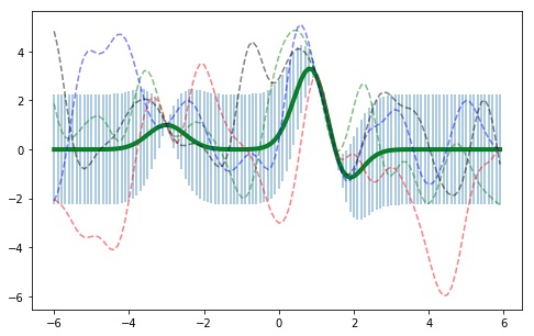
The code snippet below carries out a simple fit. The result is the plot shown at the top of this section.

from sklearn.gaussian_process.kernels import RBF, ConstantKernel as C
from sklearn.gaussian_process import GaussianProcessRegressor
import numpy as np

# Build a model
kernel = C(1.0, (1e-3, 1e3)) * RBF(10, (0.5, 2))
gp = GaussianProcessRegressor(kernel=kernel, n_restarts_optimizer=9)

# Some data
xobs = np.array([[1], [1.5], [-3]])
yobs = np.array([3, 0, 1])

# Fit the model to the data (optimize hyper parameters)
gp.fit(xobs, yobs)

# Plot points and predictions
x_set = np.arange(-6, 6, 0.1)
x_set = np.array([[i] for i in x_set])
means, sigmas = gp.predict(x_set, return_std=True)

plt.figure(figsize=(8, 5))
plt.errorbar(x_set, means, yerr=sigmas, alpha=0.5)
plt.plot(x_set, means, 'g', linewidth=4)
colors = ['g', 'r', 'b', 'k']
for c in colors:
    y_set = gp.sample_y(x_set, random_state=np.random.randint(1000))
    plt.plot(x_set, y_set, c + '--', alpha=0.5)

More details on the sklearn implementation can be found here.

Appendix C: GP Classifiers

Here, we describe how GPs are often used to fit binary classification data — data where the response variable \(y\) can take on values of either \(0\) or \(1\). The mathematics for GP Classifiers does not work out as cleanly as it does for GP Regressors. The reason is that the \(0 / 1\) response is not Gaussian-distributed, which means that the posterior is not either. To make use of the program, one approximates the posterior as normal, via the Laplace approximation.

The starting point is to write down a form for the probability of seeing a given \(y\) value at \(x\). This, ones takes as the form,

\begin{align} \tag{A8} \label{classifier} p(y \vert f(x)) = \frac{1}{1 + \exp\left (- y \times f(x)\right)}. \end{align}

This form is a natural non-linear generalization of logistic regression — see our post on this topic, here.

To proceed, the prior for \(f\) is taken to once again have form (\ref{prior}). Using this and (\ref{classifier}), we obtain the posterior for \(f\)

\begin{align} p(f \vert y) &\sim \frac{1}{1 + \exp\left (- y \times f(x)\right)} \exp \left ( - \frac{1}{2} \sum_{ij=1}^N f_i \Sigma^{-1}_{ij} f_j \right) \\ &\approx N(\mu, \Sigma^{\prime}) \tag{A9} \end{align}

Here, the last line is the Laplace / Normal approximation to the line above it. Using this form, one can easily obtain confidence intervals and samples from the approximate posterior, as was done for regressors.

Footnotes

[1] The size of the \(\sigma_i\) determines how precisely we know the function value at each of the \(x_i\) points sampled — if they are all \(0\), we know the function exactly at these points, but not anywhere else.

[2] One might wonder whether introducing more points to the analysis would change the posterior statistics for the original \(N\) points in question. It turns out that this is not the case for GPs: If one is interested only in the joint-statistics of these \(N\) points, all others integrate out. For example, consider the goal of identifying the posterior distribution of \(f\) at only a single test point \(x\). In this case, the posterior for the \(N = n+1\) points follows from Bayes’s rule,

\begin{align} \tag{f1} p(f(x_1), \ldots, f(x_n), f(x_{n+1}) \vert \{y\}) = \frac{p(\{y\} \vert f) p(f)}{p(\{y\})}. \end{align}

Now, by assumption, \(p(\{y\} \vert f)\) depends only on \(f(x_1),\ldots, f(x_n)\) — the values of \(f\) where \(y\) was sampled. Integrating over all points except the sample set and test point \(x\) gives

\begin{align} \tag{f2} &p(f(x_1), \ldots, f(x_{n+1}) \vert \{y\}) =\\ & \frac{p(\{y\} \vert f(x_1),\ldots,f(x_n))}{p(\{y\})} \int p(f) \prod_{i \not \in \{x_1, \ldots, x_N\}} df_i \end{align}

The result of the integral above is a Normal distribution — one with covariance given by the original covariance function evaluated only at the points \(\{x_1, \ldots, x_{N} \}\). This fact is proven in our post on Normal distributions — see equation (22) of that post, here. The result implies that we can get the correct sampling statistics on any set of test points, simply by analyzing these alongside the sampled points. This fact is what allows us to tractably treat the formally-infinite number of degrees of freedom associated with GPs.

[3] We have a prior post illustrating this point — see here.

[4] The marginal likelihood is equal to the denominator of (\ref{Bayes}), which we previously ignored.

[5] We made this gif through adapting the skopt tutorial code, here.

[6] For the free text by Rasmussen and Williams, see here.

Jonathan Landy Jonathan grew up in the midwest and then went to school at Caltech and UCLA. Following this, he did two postdocs, one at UCSB and one at UC Berkeley. His academic research focused primarily on applications of statistical mechanics, but his professional passion has always been in the mastering, development, and practical application of slick math methods/tools. He currently works as a data-scientist at Stitch Fix.