Daily traffic patterns can be decomposed into a historic average plus fluctuations from this average.
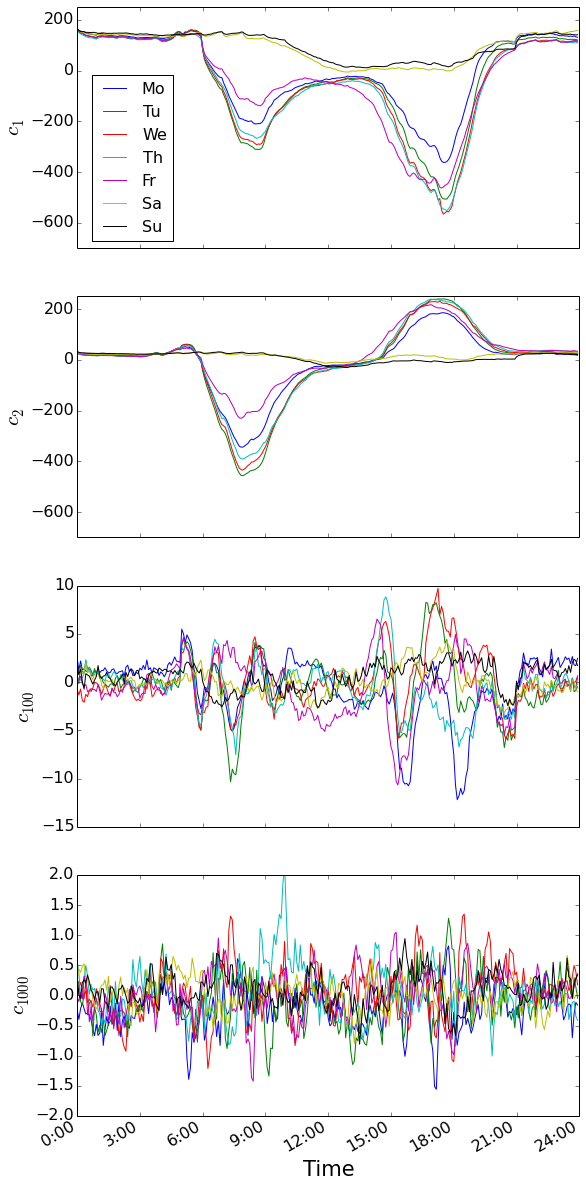
Here, we examine the daily dynamics of traffic as a function of weekday to provide the first piece of this puzzle. To do this, we average the time-dependent scores \(c_i(t)\) for each day of the week (see plot to the right).
As discussed previously, modes one and two are general indicators of overall traffic density and directional commuter density, respectively. Interestingly, we can clearly see systematic deviations in these two mode amplitudes across the days of the week: During rush hour, Mondays and Fridays have generally lower levels of traffic by both measures - most likely a consequence of people taking three-day weekends. In addition, if you look closely, you can actually see evidence of slackers taking off early on Friday afternoons.
Examining higher modes, the average signal dies away, eventually being lost in the noise. The final two panels in the figure have different y-axis scales - zoomed in to show the signal-to-noise ratio. By mode 100 the signal is already quite weak, but systematic deviations from zero can still be seen above the noise. However, by mode 1000, there are no systematic or significant deviations from zero. These minor principal components likely represent rare events such as traffic accidents and thus are not reflected at all in the daily averages.
Is the historic average the best we can do for prediction? To answer this we must examine the predictability of the fluctuations away from these means. Here, we examine the autocorrelation\(^1\) of the fluctuations from the mean to find the memory time scale of each principal component’s fluctuation memory. This quantity characterizes the time scale over which we can extrapolate each amplitude deviation into the future (see plot\(^2\) below). The time scale of initial decay of the correlation decreases monotonically with the mode index - the modes that capture the most variance have the longest memory: several hours.
This is excellent news: we can do better than just using the historic traffic patterns. We can, in fact, project fluctuations away from the historic average several hours into the future and expect some improvement.
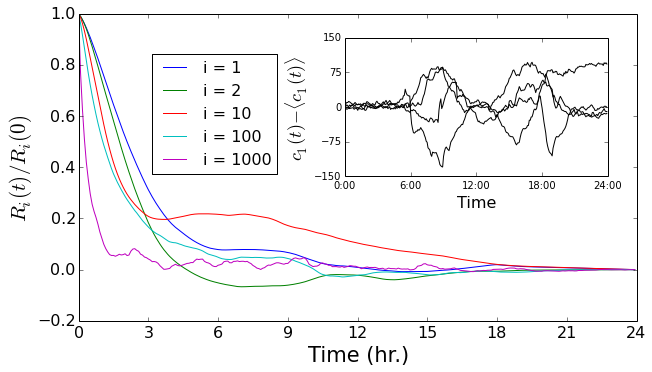
[1] The autocorrellation: The autocorrelation of a stochastic signal is a measure of its memory. In this particular case, \(R_{i}(t) \propto \mathbb{E}[\Delta c_i(s) \cdot \Delta c_i(s+t)]\) where the expectation value is over \(s\) and \(\Delta c_i(t) = c_i(t) - \langle c_i(t) \rangle\).
[2] On this plot: The plot shown is for Tuesdays — other days have exhibit similar characteristics. Note that mode 2 takes on negative autocorrelation values for a period of time (\(t =\) 6-9 hours). This is not surprising since mode 2, being an “odd” mode, tends to reverse sign between rush hours. The inset shows a few mean-subtracted signals for the first mode, ($\Delta c_1(t) $ above). The long-time correlations of these fluctuations are apparent here.
 Dustin got a B.S in Engineering Physics from the Colorado School of Mines (Golden, CO) before moving to UC Santa Barbara for graduate school. There he became interested in Soft Condensed Matter Physics and Polymer Physics, studying the interaction between single DNA molecules and salt ions. After a brief postdoc at UC San Diego studying the physics of bacterial growth, Dustin decided to move into the data science business for good - he is now a Quantitative Analyst at Google in Mountain View.