Support Vector Machines for classification

To whet your appetite for support vector machines, here’s a quote from machine learning researcher Andrew Ng:

“SVMs are among the best (and many believe are indeed the best) ‘off-the-shelf’ supervised learning algorithms.”

Professor Ng covers SVMs in his excellent Machine Learning MOOC, a gateway for many into the realm of data science, but leaves out some details, motivating us to put together some notes here to answer the question:

“What are the support vectors in support vector machines?”

We also provide python (https://github.com/EFavDB/svm-classification/blob/master/svm.ipynb) using scikit-learn’s svm module to fit a binary classification problem using a custom kernel, along with code to generate the (awesome!) interactive plots in Part 3.

This post consists of three sections:

Part 1 sets up the problem from a geometric point of view and then shows how it can be framed as an optimization problem.
Part 2 transforms the optimization problem and uncovers the support vectors in the process.
Part 3 discusses how kernels can be used to separate non-linearly separable data.

Part 1: Defining the margin

Maximizing the margin

The figure below is a binary classification problem (points labeled $y_i = \pm 1$) that is linearly separable.

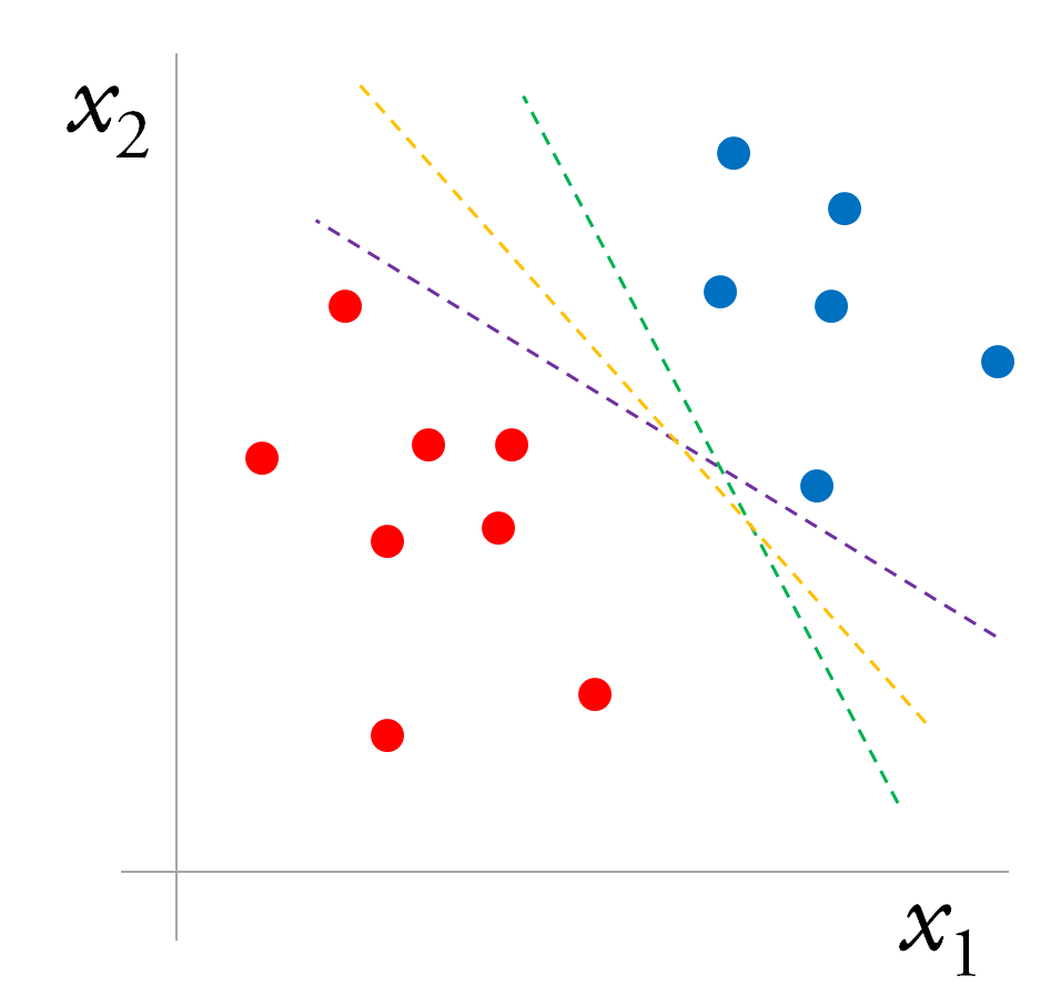
There are many possible decision boundaries that would perfectly separate the two classes, but an SVM will choose the line in 2-d (or “hyperplane”, more generally) that maximizes the margin around the boundary.

Intuitively, we can be very confident about the labels of points that fall far from the boundary, but we’re less confident about points near the boundary.

Formulating the margin with geometry

Any point $\boldsymbol{x}$ lying on the separating hyperplane satisfies: $\boldsymbol{w} \cdot \boldsymbol{x} + b = 0$ $\boldsymbol{w}$ is the vector normal to the plane, and $b$ is a constant that describes how much the plane is shifted relative to the origin. The distance of the plane from the origin is $b / \| \boldsymbol{w} \|$.

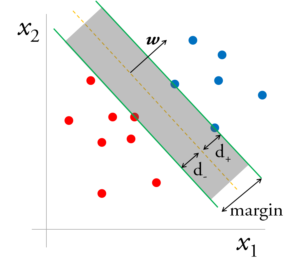
Now draw parallel planes on either side of the decision boundary, so we have what looks like a road, with the decision boundary as the median, and the additional planes as gutters. The margin, i.e. the width of the road, is ($d_+ + d_-$) and is restricted by the data points closest to the boundary, which lie on the gutters.

The half-spaces bounded by the planes on the gutters are:

$\boldsymbol{w} \cdot \boldsymbol{x} + b \geq +a$, for $y_i = +1$

$\boldsymbol{w} \cdot \boldsymbol{x} + b \leq -a$, for $y_i = -1$

These two conditions can be put more succinctly:

$y_i (\boldsymbol{w} \cdot \boldsymbol{x} + b) \geq a, \forall \; i$

Some arithmetic leads to the equation for the margin:

$d_+ + d_- = 2a / \| \boldsymbol{w} \|$

Without loss of generality, we can set $a=1$, since it only sets the scale (units) of $b$ and $\boldsymbol{w}$. So to maximize the margin, we have to maximize $1 / \| \boldsymbol{w} \|$. However, this is an unpleasant (non-convex) objective function. Instead we minimize $\| \boldsymbol{w}\|^2$, which is convex.

The optimization problem

Maximizing the margin boils down to a constrained optimization problem: minimize some quantity $f(w)$, subject to constraints $g(w,b)$. This optimization problem is particularly nice because it is convex; the objective $\| \boldsymbol{w}\|^2$ is convex, as are the constraints, which are linear.

In other words, we are faced with a quadratic programming problem. The standard format of the optimization problem for the separable case is

$$\tag{1} \label{problem} \begin{align} \text{minimize} \quad & f(w) \equiv (1/2) \| \boldsymbol{w}\|^2 \ \text{subject to} \quad & g(w,b) \equiv -y_i (\boldsymbol{w} \cdot \boldsymbol{x} + b) + 1 \leq 0, \; i = 1 \ldots m \end{align} $$

Before we address how to solve this optimization problem in Part 2, let’s first consider the case when data is non-separable.

Soft margin SVM: the non-separable problem and regularization

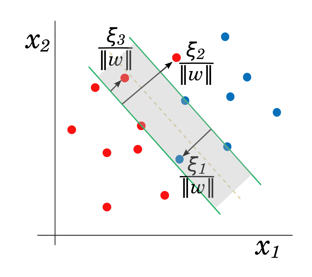
For non-separable data, we relax the constraints in (\ref{problem}) while penalizing misclassified points via a cost parameter $C$ and slack variables $\xi_i$ that define the amount by which data points are on the wrong side of the margin.

$$\tag{2} \label{regularization} \begin{align} \text{minimize} \quad & (1/2) \| \boldsymbol{w}\|^2 + C \sum_i^m \xi_i \\ \text{subject to} \quad & y_i (\boldsymbol{w} \cdot \boldsymbol{x} + b) \geq 1 - \xi_i, \; i = 1 \ldots m \\ & \xi_i \geq 0, \quad i = 1 \ldots m \end{align} $$

A large penalty — large $C$ — for misclassifications will lead to learning a lower bias, higher variance SVM, and vice versa for small $C$.

The soft margin is used in practice; even in the separable case, it can be desirable to allow tradeoffs between the size of the margin and number of misclassifications. Outliers can skew the decision boundary learned by (\ref{problem}) towards a model with small margins + perfect classification, in contrast to a possibly more robust model learned by (\ref{regularization}) with large margins + some misclassified points.

Part 2: Solving the optimization problem

In Part 1, we showed how to set up SVMs as an optimization problem. In this section, we’ll see how the eponymous support vectors emerge when we rephrase the minimization problem as an equivalent maximization problem.

To recap: Given $m$ training points that are labeled $y_i = \pm 1$, our goal is to maximize the margin of the hyperplane defined by $\boldsymbol{w} \cdot \boldsymbol{x} + b = 0$.

We’ll use the separable case (\ref{problem}) as our starting point, but the steps in the procedure and final result are similar for the non-separable case (also worked out in ref [3]).

The Lagrangian formulation

How do we solve this optimization problem? Minimizing a function without constraints is probably familiar: set the derivative of the function (the objective) to zero and solve.

With constraints, the procedure is similar to setting the derivative of the objective equal to zero. Instead of taking the derivative of the objective itself, however, we’ll operate on the Lagrangian $\mathcal{L}$, which combines the objective and inequality constraints into one function:

$$\tag{3} \label{Lagrangian} \mathcal{L}(w,b,\alpha) = f(w) + \sum_i^m \alpha_i g_i(w,b) $$

We’ve just introduced additional variables $\alpha_i$, Lagrange multipliers, that make it easier to work with the constraints (see Wikipedia about the method of Lagrange multipliers). Note, a more general form for the Lagrangian would include another summation term in (\ref{Lagrangian}) to uphold equality constraints. Since there are only inequality constraints here, we’ll omit the extra term.

Constructing the dual problem

Much of the following discussion is based off ref [2], which has a nice introduction to duality in the context of SVMs.

First, let’s make the following observation:

$$\tag{Obs. 1} \max_{\alpha} \mathcal{L}(w,b,\alpha) = \begin{cases} f(w), & \text{if } g_i(w) \leq 0, \; \text{(constraints satisfied)} \\ \infty, & \text{if } g_i(w) \gt 0, \; \text{(constraints violated)} \end{cases} $$

Basically, if any constraint $j$ is violated, i.e. $g_j(w) > 0$, then the Lagrange multiplier $\alpha_j$ that is multiplying $g_j(w)$ can be made arbitrarily large ($\rightarrow \infty$) in order to maximize $\mathcal{L}$.

On the other hand, if all the constraints are satisfied, $g_i(w) \leq 0$ $\forall \; i$, then $\mathcal{L}$ is maximized by setting the $\alpha_i$s that are multiplying negative quantities equal to zero. However, Lagrangian multipliers multiplying $g_i(w)$ that satisfy the constraints with equality, $g_i(w) = 0$, can be non-zero without diminishing $\mathcal{L}$.

The last statement amounts to the property of “complementary slackness” in the Karush-Kuhn-Tucker conditions for the solution:

$$\tag{4} \label{complementarity} \alpha_i g_i(w) = 0 $$

Recall from the original geometric picture: only a few points lie exactly on the margins, and those points are described by $g_i(w) = 0$ (and thus have non-zero Lagrange multipliers). The points on the margin are the support vectors.

Next, we make use of the Max-Min inequality:

$$ \max_{\alpha} \min_{w,b} \mathcal{L}(w,b,\alpha) \leq \min_{w,b} \max_{\alpha} \mathcal{L}(w,b,\alpha) $$

This inequality is an equality under certain conditions, which our problem satisfies (convex $f$ and $g$). The left side of the inequality is called the dual problem, and the right side is the primal problem.

Now we can put it all together: Observation 1 tells us that solving the right side (primal problem) of the Max-Min inequality is the same as solving the original problem. Because our problem is convex, solving the left side (dual) is equivalent to solving the primal problem by the Max-Min inequality.

Thus we’re set to approach the solution via the dual problem, which is useful for dealing with nonlinear decision boundaries.

Solving the dual problem

The dual problem to solve is $\max_{\alpha} \min_{w,b} \mathcal{L}(w,b,\alpha)$, subject to constraints* on the Lagrange multipliers: $\alpha_i \geq 0$.

Let’s work out the inner part of the expression explicitly. We obtain $\min_{w,b} \mathcal{L}(w,b,\alpha)$ by setting:

$$ \nabla_\boldsymbol{w} \mathcal{L} = 0; \quad \partial_b \mathcal{L} = 0 $$

These equations for the partial derivatives give us, respectively:

$$ \boldsymbol{w} = \sum_i \alpha_i y_i \boldsymbol{x}_i; \quad \sum_i \alpha_i y_i = 0 $$

$\boldsymbol{w}$ is a linear combination of the coordinates of the training data. Only the support vectors, which have non-zero $\alpha_i$, contribute to the sum. To predict the label for a new test point $\boldsymbol{x_t}$, simply evaluate the sign of

$$\tag{5} \label{testing} \boldsymbol{w} \cdot \boldsymbol{x} + b = \sum_i \alpha_i y_i \boldsymbol{x}_i \cdot \boldsymbol{x_t} + b $$

where b can be computed from the KKT complementarity condition (\ref{complementarity}) by plugging in the values for any support vector. The equation for the separating hyperplane is entirely determined by the support vectors.

Plugging the last two equations into $\mathcal{L}$ leads to the dual formulation of the problem $ \max_{\alpha} \mathcal{L}_D$:

$$\tag{6} \label{dual} \begin{align} \max_{\alpha} \quad & \sum_i \alpha_i - (1/2) \sum_{i,j} \alpha_i \alpha_j y_i y_j \boldsymbol{x_i} \cdot \boldsymbol{x_j} \\ \text{subject to} \quad & \alpha_i \geq 0, \; i = 1 \ldots m \\ & \sum_i \alpha_i y_i = 0 \end{align} $$

The dual for the non-separable primal Lagrangian (\ref{regularization}) — derived using the same procedure we just followed — looks just like the dual for the separable case (\ref{dual}), except that the Lagrange multipliers are bounded from above by the regularization constant: $0 \leq \alpha_i \leq C$. Notably, the slack variables $\xi_i$ do not appear in the dual of the soft margin SVM.

The dual (called the Wolfe dual) is easier to solve because of the simpler form of its inequality constraints and is the form used in algorithms such as the Sequential Minimal Optimization algorithm, which is implemented in the popular SVM solver, LIBSVM. The key feature of the dual is that training vectors only appear as dot products $\boldsymbol{x_i} \cdot \boldsymbol{x_j}$. This property allows us to generalize to the nonlinear case via the “kernel trick” discussed in Part 3 of this post.

Some of you may be familiar with using Lagrangian multipliers to optimize some function $f(\boldsymbol{x})$ subject to equality constraints $g(\boldsymbol{x}) = 0$, in which case the Lagrangian multipliers are unconstrained. The Karush-Kuhn-Tucker conditions generalize the method to include inequality constraints $g(\boldsymbol{x}) \leq 0$, which results in additional constraints on the associated Lagrangian multipliers (as we have here).

Part 3: Kernels

Data that is not linearly separable in the original input space may be separable if mapped to a different space. Consider the following example of nonlinearly separable, two-dimensional data:

However, if we map the 2-d input data $\boldsymbol{x} = (x, y)$ to 3-d feature space by a function $\Phi(\boldsymbol{x}) = (x,\; y,\; x^2 + y^2)$, the blue and red points can be separated with a plane in the new (3-d) space. See the plot below of the decision boundary, the mapped points, as well as the the original data points in the x-y plane. Drag the figure to rotate it, or zoom in and out with your mouse wheel!

Code to generate and fit the data in this example with scikit-learn’s SVM module, as well as code to create the plot.ly interactive plots above, is available in IPython notebooks on github.

From maps to kernels

So how do we incorporate mapping the data into the formulation of the problem?

Recall that the data appears as a dot product in the dual Lagrangian (\ref{dual}). If we decide to train an SVM on the mapped data, then the dot product of the input data in (\ref{dual}) is replaced by the dot product of the mapped data: $\boldsymbol{x_i} \cdot \boldsymbol{x_j} \rightarrow \Phi(\boldsymbol{x_i}) \cdot \Phi(\boldsymbol{x_j})$

The kernel is simply the dot product of the mapping functions. In the example above, the inner product of the mapping function is an instance of a polynomial kernel:

$$ K(x_i, x_j) = \Phi(\boldsymbol{x_i}) \cdot \Phi(\boldsymbol{x_j}) = x_i x_j + y_i y_j + (x_i^2 + y_i^2)(x_j^2 + y_j^2) $$

In practice, we work directly with the kernel $K(x_i, x_j)$ rather than explicitly computing the map of the data points**. Computing the kernel directly allows us to sidestep the computationally expensive operation of mapping data to a high dimensional space and then taking a dot product (see ref [2] for examples comparing computational times of the two methods).

Using a kernel, the second term in the objective of the dual problem (\ref{dual}) becomes

$$ \sum_{i,j} \alpha_i \alpha_j y_i y_j K(x_i, x_j) $$

The kernel also appears in the evaluation of (\ref{testing}) to predict the classification of a test point $\boldsymbol{x_t}$:

$$\tag{8} \label{testingKernel} sgn \left(\sum_i \alpha_i y_i K(x_i, x_t) + b \right) $$

Which functions are valid kernels to use in the kernel trick? i.e. given $K(x_i, x_j)$, does some feature map $\Phi$ exist such that $K(x_i, x_j)=\Phi(\boldsymbol{x_i}) \cdot \Phi(\boldsymbol{x_j})$ for any $i,\ j$? Mercer’s condition states that a necessary and sufficient condition for $K$ to be a valid kernel is that it is symmetric and positive semi-definite$^\dagger$.

Some popular kernels are:

$$ \begin{align} \text{polynomial:} & \quad (\boldsymbol{x_i} \cdot \boldsymbol{x_j} + c)^p \\ \text{Gaussian radial basis function:} & \quad \exp(-\|\boldsymbol{x_i} - \boldsymbol{x_j} \|^2/2\sigma^2) \end{align} $$

The optimal parameters for the degree of the polynomial $p$ and spread of the Gaussian $\sigma$ (as well as the regularization parameter) are determined by cross-validation. Computing the above kernels takes $\mathcal{O}(d)$ time, where $d$ is the dimension of the input space, since we have to evaluate $\boldsymbol{x_i} \cdot \boldsymbol{x_j}$ in the polynomial kernel and $\boldsymbol{x_i} - \boldsymbol{x_j}$ in the Gaussian kernel.

Comparing runtimes of linear and nonlinear kernels

The computational complexity for classification/prediction, i.e. at test time, can be obtained by eyeballing (\ref{testing}) and (\ref{testingKernel}). Let $d$ be the dimension of the input space and $n$ be the size of the training set, and assume the number of support vectors $n_S$ is some fraction of $n$, $n_S \sim \mathcal{O}(n)$.

In the case of working with the linear kernel/original input space, $\boldsymbol{w}$ can be explicitly evaluated to obtain the separating hyperplane parameters, so that classification in (\ref{testing}) takes $\mathcal{O}(d)$ time. On the other hand, with the kernel trick, the hyperplane parameters are not explicitly evaluated. Assume calculating a kernel takes $\mathcal{O}(d)$ time, cf. the polynomial and Gaussian kernels; then test time for a nonlinear $K$ in (\ref{testingKernel}) takes $\mathcal{O}(nd)$ time.

Estimating the computational complexity for training is complicated, so we defer the discussion to refs [4a, 4b] and simply state the result: training for linear kernels is $\mathcal{O}(nd)$ while training for nonlinear kernels using the Sequential Minimal Optimization algorithm is $\mathcal{O}(n^2)$ to $\mathcal{O}(n^3)$ (dependent on the regularization parameter $C$), making nonlinear kernel SVMs impractical for larger datasets (a couple of 10,000 samples according to scikit-learn).

** More than one mapping and feature space (dimension) may exist for a particular kernel. See section 4 of ref [1] for examples.

$^\dagger$ See ref [2] for a simple proof in terms of the Kernel (Gram) matrix, i.e. the kernel function evaluated on a finite set of points.

Discussion

We’ve glimpsed the elegant theory behind the construction of SVMs and seen how support vectors pop out of the mathematical machinery. Geometrically, the support vectors are the points lying on the margins of the decision boundary.

How about using SVMs in practice?

In his Coursera course, Professor Ng recommends linear and Gaussian kernels for most use cases. He also provides some rules of thumb (based on the current state of SVM algorithms) for different sample sizes $n$ and input data dimension/number of features $d$, restated here:

case method $n$ $d$

$n \ll d$, e.g. genomics, bioinformatics data linear kernel SVM or logistic regression 10 - 1000 10,000 $n$ intermediate, $d$ small Gaussian kernel SVM 10 - 10,000 1 - 1000 $n \gg d$ create features, then linear kernel SVM or logistic regression 50,000+ 1 - 1000

The creators of the LIBSVM and LIBLINEAR packages also provide a user’s guide for novices, which includes a study of when to use linear instead of radial basis function kernels. They recommend linear SVMs when $d$ and $n$ are both large, often encountered in document classification problems where bag-of-words approaches can generate huge numbers of features (in their example $n =$ 20,000, $d =$ 47,000).

The idea is that if the input data is already high-dimensional, then it shouldn’t be necessary to apply nonlinear transformations to it in order to obtain a separating hyperplane.

Tip: LIBLINEAR is specifically optimized for linear kernels and should be used instead of LIBSVM in the linear case.