Textbook proofs of the duality theorem often apply abstract arguments that offer little tangible insight into the relationship between a linear program and its dual. Here, we map the general linear program onto a simple mechanics problem. In this context, the significance of the theorem is relatively clear.
The general linear program and its dual
The goal of a linear program is to optimize a linear objective function subject to some linear constraints. By introducing slack and other auxiliary variables, the general linear program can be expressed as [1]
Here, the optimization is over \(\textbf{x} \in \mathbb{R}_n\), \(A\) is a given \(m \times n\) real matrix, \(\textbf{b}\) and \(\textbf{c}\) are given real vectors, and the inequality holds component-wise. Any \(\textbf{x}\) that satisfies the inequality constraints above is called a feasible solution to (\ref{primal}) and if a point can be found with finite components that optimizes the objective it is called an optimal solution. Associated with (\ref{primal}) is the dual linear program,
The optimization here is over \(\textbf{w} \in \mathbb{R}_m\), and \(A\), \(\textbf{b}\), and \(\textbf{c}\) are the same variables present in (\ref{primal}). In this post, we apply some simple ideas from classical mechanics to prove the following theorem, one of the central results connecting the two linear programs above:
Duality theorem
If (\ref{primal}) has an optimal solution at \(\textbf{x}^*\), then (\ref{dual}) will also have an optimal solution at some point \(\textbf{w}^*\), and these points satisfy
That is, the optimal objectives of (\ref{primal}) and (\ref{dual}) agree.
Proof:
To begin we assume that \(\textbf{x}^*\) is an optimal solution to (\ref{primal}). We also assume for simplicity that (i) we have chosen a coordinate system so that \(\textbf{x} = \textbf{0}\) is a feasible solution of (\ref{primal}) and that (ii) each row \(\hat{\textbf{A}}_i\) of \(A\) has been normalized to unit length.
Next, we introduce a physical system relevant to (\ref{primal}) and (\ref{dual}): We consider a mobile point particle that interacts with a set of \(m\) fixed walls, all sitting in \(\mathbb{R}_n\). The particle’s coordinate \(\textbf{x}_p\) is initially set to \(\textbf{x}_p = \textbf{0}\). The fixed \(i\)-th wall sits at those points \(\textbf{x}\) that satisfy \(\hat{\textbf{A}}_i \cdot \textbf{x} = b_i\). We take the force on the particle from wall \(i\) to have two parts: (i) a constant, long range force, \(w_i \hat{\textbf{A}}_i\), normal to the wall, and (ii) a “hard core” force, \(-n_i(\textbf{x}_p) \hat{\textbf{A}}_i\), also normal to the wall. The hard core force makes the wall impenetrable to the particle, but otherwise allows the particle to move freely: Its magnitude is zero when the particle does not touch the wall, but on contact it scales up to whatever value is needed to prevent the particle from passing through it.
To relate the physical system to our linear programs, we’ll require \(\textbf{x}_p\) to be a feasible solution to (\ref{primal}) and the vector of long range force magnitudes \(\textbf{w}\) to be a feasible solution to (\ref{dual}). A point \(\textbf{x}_p\) is a feasible solution to (\ref{primal}) if and only if the particle is within the interior space bounded by the set of walls. Further, the equality constraint of (\ref{dual}) is equivalent to the condition that all feasible \(\textbf{w}\) result in a total long range force acting on the particle of \(\sum_i w_i \hat{\textbf{A}}_i = \textbf{c}\). The non-negativity condition on feasible \(\textbf{w}\) vectors in (\ref{dual}) further requires that the long range forces each be either attractive or zero. A simple example of the sort of physical system we’ve described here is shown in Fig. 1a.
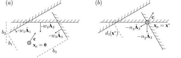
Fig. 1: An example system: (a) A particle at \(\textbf{x}_p=\textbf{0}\) interacts with three walls. The total long range force on the particle is \(\sum_i w_i \hat{\textbf{A}}_i = \textbf{c}\). (b) The particle sits at its long range potential minimum, \(\textbf{x}^*\), with walls \(2\) and \(3\) “binding”. The hard core normal forces from these walls must point inward and sum to \(-\textbf{c}\) — otherwise, there would be a net force on the particle, and it would continue to move, but that won’t happen once it sits at its potential minimum. Wall \(1\) is not binding and is now a distance \(d_1(\textbf{x}^*)\) away from the particle. This results in a positive difference between the dual and primal objectives (\ref{gap}), unless we can find a feasible \(\textbf{w}\) for which \(w_1=0\). Setting \(\textbf{w}^* = \textbf{n}(\textbf{x}^*)\) — the vector of hard-core normal force magnitudes at \(\textbf{x}^*\) — provides such a solution. This is non-negative, zero for non-binding walls, and results in a total long range force of \(\textbf{c}\) — a consequence of the point above that the particle must remain at rest at its potential minimum. This choice for \(\textbf{w}\) optimizes (\ref{dual}) and gives an objective matching that of (\ref{primal}) at \(\textbf{x}^*\).
When we assert the conditions above, the potential associated with the long range forces in our physical system ends up being related to the objective functions of (\ref{primal}) and (\ref{dual}). Up to a constant, the potential of a force \(\textbf{f}(\textbf{x})\) is defined to be [2]
In our case, the long range force between the wall \(i\) and the particle is a constant and normal to the wall. Its potential is therefore simply
where
This is the perpendicular distance between the particle and the wall \(i\). The physical significance of (\ref{potential_i}) is that it is the total energy it takes to separate the particle from wall \(i\) by a distance \(d_i\), working against the attractive force \(w_i\). Notice that if we plug (\ref{perp_distance}) into (\ref{potential_i}), the total long range potential at \(\textbf{x}_p\) can be written as
Here, we have used one of the feasibility conditions on \(\textbf{w}\) to get the last line. The right side of (\ref{potential_as_objective_difference}) is the difference between the dual and primal objectives. This will be minimized at the feasible point \(\textbf{x}_p\) that maximizes \(\textbf{c}\cdot \textbf{x}_p\) — the primal objective — and at that feasible \(\textbf{w}\) that minimizes \(\textbf{w}^T \cdot \textbf{b}\) — the dual objective. In other words, we see that both our programs independently contribute to the common goal of minimizing the particle’s long range potential, (\ref{potential_as_objective_difference}), subject to our system’s constraints.
The last preperatory remark we must make relates to the fact that we have assumed that \(\textbf{x}^*\) is an optimal solution to (\ref{primal}) — i.e., it is a point that is as far “down” in the \(\textbf{c}\) direction as possible within the feasible set. This must mean that \(\textbf{x}^*\) sits somewhere at the boundary of the primal feasible set, with some of the constraints of (\ref{primal}) binding — i.e., satisfied as equalities. Further, if we place and release the particle gently at \(\textbf{x}^*\), it must stay at rest as it can fall no further — just as a particle acted on by gravity stays at rest when it is placed in the bottom of a bucket. To stay at rest, there must be no net force on the particle, which means that the hard core normal forces \(-n_i \hat{\textbf{A}}_i\) from the binding walls at \(\textbf{x}^*\) must sum to exactly \(-\textbf{c}\), fully countering the constant long range force. The set of forces acting on the particle at \(\textbf{x}^*\) is illustrated Fig. 1b for our simple example.
To complete the argument, we note that the long range potential at \(\textbf{x}^*\) is given from (\ref{potential_as_objective_difference}) by
This is non-negative because \(\textbf{w} \geq \textbf{0}\) and \(d_i(\textbf{x}^*) >0\) for each non-binding wall. It follows that the dual objective is always bounded from below by the optimal primal objective. Further, the gap between the two — the left side of (\ref{gap}) — can only be zero if the long range interaction strengths are zero for each non-binding wall at \(\textbf{x}^*\) — i.e., if the particle is not actually attracted to the walls that are not binding at \(\textbf{x}^*\). The vector \(\textbf{n}(\textbf{x}^*)\) of hard core normal force magnitudes at \(\textbf{x}^*\) provides such a solution for \(\textbf{w}\): This is a feasible \(\textbf{w}\) because it is non-negative and results in normal forces that sum to \(\textbf{c}\). Further, it is non-zero only for the binding constraints. It follows that \(\textbf{w}^* = \textbf{n}(\textbf{x}^*)\) gives an optimal solution to the dual, at which point its objective matches that of the optimal primal solution. This argument is summarized in the caption to Fig. 1.
References
[1] Matousek, J., and Ga ̈rtner, B. Understanding and using linear programming. Springer (2007)
[2] Marion, Jerry B. Classical dynamics of particles and systems. Academic Press, (2013).
 Jonathan grew up in the midwest and then went to school at Caltech and UCLA. Following this, he did two postdocs, one at UCSB and one at UC Berkeley. His academic research focused primarily on applications of statistical mechanics, but his professional passion has always been in the mastering, development, and practical application of slick math methods/tools. He currently works as a data-scientist at Stitch Fix.