Machine learning for facial recognition

A guest post, contributed by Damien Ramunno-Johnson (LinkedIn, bio-sketch)

Introduction

The ability to identify faces is a skill that people develop very early in life and can apply almost effortlessly. One reason for this is that our brains are very well adapted for pattern recognition. In contrast, facial recognition can be a somewhat difficult problem for computers. Today, given a full frontal image of a face, computer facial recognition software works well. However, problems can arise given large camera angles, poor lighting, or exaggerated facial expressions: Computers have a ways to go before they catch up with us in this arena.

Although facial recognition algorithms remain imperfect, the methods that exist now are already quite useful and are being applied by many different companies. Two examples, first up Facebook: When you upload pictures to their website, it will now automatically suggest names for the people in your photos. This application is well-suited for machine learning for two reasons. First, every tagged photo already uploaded to the site provides labeled examples on which to train an algorithm, and second, people often post full face images in decent lighting. A second example is provided by Google’s Android phone OS, which has a face unlock mode. To get this to work, you first have to train your phone by taking images of your face in different lighting conditions and from different angles. After training, the phone can attempt to recognize you. This is another cool application that also often works well.

In this post, we’re going to develop our own basic facial learning algorithm. We’ll find that it is actually pretty straightforward to set one up that is reasonably accurate. Our post follows and expands upon the tutorial found here.

Loading packages and data

from __future__ import print_function

from time import time
import matplotlib.pyplot as plt

from sklearn.cross_validation import train_test_split
from sklearn.datasets import fetch_lfw_people
from sklearn.grid_search import GridSearchCV
from sklearn.metrics import classification_report
from sklearn.metrics import confusion_matrix
from sklearn.decomposition import RandomizedPCA
from sklearn.svm import SVC
import pandas as pd
%matplotlib inline

The sklearn function fetch_lfw_people, imported above, will download the data that we need, if not already present in the faces folder. The dataset we are downloading consists of a set of preprocessed images from Labeled Faces in the Wild (LFW), a database designed for studying unconstrained face recognition. The data set contains more than 13,000 images of faces collected from the web, each labeled with the name of the person pictured. 1680 of the people pictured have two or more distinct photos in the data set.

In our analysis here, we will impose two conditions.

1. First, we will only consider folks that have a minimum of 70 pictures in the data set.
2. We will resize the images so that they each have a 0.4 aspect ratio.

print('Loading Data')
people = fetch_lfw_people(
'./faces', min_faces_per_person=70, resize=0.4)
print('Done!')
>>
Loading Data
Done!

The object people contains the following data.

1. people.data: a numpy array with the shape(n_samples, h*w), each row corresponds to a unravelled face.
2. people.images: a numpy array with the shape(n_samples, h, w), where each row corresponds to a face. The remaining indices here contain gray-scale values for the pixels of each image.
3. people.target: a numpy array with the shape(n_samples), where each row is the label for the face.
4. people.target_name: a numpy array with the shape(n_labels), where each row is the name for the label.

For the algorithm we will be using, we don’t need the relative position data, so we will use the unraveled people.data.

#Find out how many faces we have, and
#the size of each picture from.
n_samples, h, w = people.images.shape

X = people.data
n_features = X.shape[1]

y = people.target
target_names = people.target_names
n_classes = target_names.shape[0]

print("Total dataset size:")
print("n_images: %d" % n_samples)
print("n_features: %d" % n_features)
print("n_classes: %d" % n_classes)
>>
Total dataset size:
n_images: 1288
n_features: 1850
n_classes: 7

Looking above we see that our dataset currently has 1288 images. Each image has 1850 pixels, or features. We also have 7 classes, meaning images of 7 different people.

Data segmentation and dimensional reduction

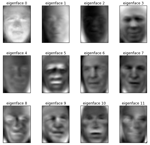
At this point we need to segment our data. We are going to use train_test_split, which will take care of splitting our data into random training and testing data sets. Next, we note that we have a lot of features and that there are advantages to having fewer: First, the computational cost is reduced. Second, having fewer features reduces the data’s dimension which can also reduce the complexity of the model and help avoid overfitting. Instead of dropping individual pixels outright, we will carry out a dimensional reduction via a Principle Component Analysis PCA. PCA works by attempting to represent the variance in the training data with as few dimensions as possible. So instead of dropping features, as we did in our wearable sensor example analysis, here we will compress features together, and then use only the most important feature combinations. When this is done to images, the features returned by PCA are commonly called eigenfaces (some examples are given below).

The function we are going to use to carry out our PCA is RandomizedPCA. We’ll keep the top 150 eigenfaces, and we’ll also whiten the data — ie normalize our new, principal component feature set. The goal of whitening is to make the input less redundant. Whitening is performed by rotating into the coordinate space of the principal components, dividing each dimension by square root of variance in that direction (giving the feature unit variance), and then rotating back to pixel space.

# split into a training and testing set
X_train, X_test, y_train, y_test = train_test_split(
X, y, test_size=0.25)

# Compute the PCA (eigenfaces) on the face dataset
n_components = 150

pca = RandomizedPCA(
n_components=n_components, whiten=True).fit(X_train)

eigenfaces = pca.components_.reshape((n_components, h, w))
X_train_pca = pca.transform(X_train)

Visualizing the eigenfaces

Let’s now take a moment to examine the dataset’s principal eigenfaces: the set of images that we will project each example onto to obtain independent features. To do that we will use the following helper function to make life easier — visual follows.

# A helper function to make plots of the faces
def plot_gallery(images, titles, h, w, n_row=3, n_col=4):
plt.figure(figsize=(1.8 * n_col, 2.4 * n_row))
plt.subplots_adjust(bottom=0, left=.01, right=.99,
top=.90, hspace=.35)
for i in range(n_row * n_col):
plt.subplot(n_row, n_col, i + 1)
plt.imshow(images[i].reshape((h, w)), cmap=plt.cm.gray)
plt.title(titles[i], size=12)
plt.xticks(())
plt.yticks(())

# Plot the gallery of the most significative eigenfaces
eigenface_titles = [
"eigenface %d" % i for i in range(eigenfaces.shape[0])]

plot_gallery(eigenfaces, eigenface_titles, h, w)

plt.show()

Training a model

Now that we have reduced the dimensionality of the data it is time to go ahead and train a model. I am going to use the same SVM and GridSearchCV method I explained in my previous post. However, instead of using a linear kernel, as we did last time, I’ll use instead a radial basis function (RBF) kernel. The RBF kernel is a good choice here since we’d like to have non-linear decision boundaries — in general, it’s a reasonable idea to try this out whenever the number of training examples outnumbers the number of features characterizing those examples. The parameter C here acts as a regularization term: Small C values give you smooth decision boundaries, while large C values give complicated boundaries that attempt to fit/accommodate all training data. The gamma parameter defines how far the influence of a single point example extends (the width of the RBF kernel).

#Train a SVM classification model

print("Fitting the classifier to the training set")
t0 = time()
param_grid = {'C': [1e3, 5e3, 1e4, 5e4, 1e5],
'gamma': [0.0001, 0.0005, 0.001, 0.005, 0.01, 0.1], }

clf = GridSearchCV(
SVC(kernel='rbf', class_weight='auto'), param_grid)
clf = clf.fit(X_train_pca, y_train)
print("done in %0.3fs" % (time() - t0))
print("Best estimator found by grid search:")
print(clf.best_estimator_)

>>
Fitting the classifier to the training set
done in 16.056s
Best estimator found by grid search:
SVC(C=1000.0, cache_size=200, class_weight='auto', coef0=0.0,
degree=3, gamma=0.001, kernel='rbf', max_iter=-1,
probability=False, random_state=None, shrinking=True,
tol=0.001, verbose=False)

Model validation

That’s it for training! Next we’ll validate our model on the testing data set. Below, we first use our PCA model to transform the testing data into our current feature space. Then, we apply our model to make predictions on this set. To get a feel for how well the model is doing, we print a classification_report and a confusion matrix.

#Quantitative evaluation of the model quality on the test set
#Validate the data
X_test_pca = pca.transform(X_test)
y_pred = clf.predict(X_test_pca)

print(classification_report(
y_test, y_pred, target_names=target_names))

print('Confusion Matrix')
#Make a data frame so we can have some nice labels
cm = confusion_matrix(y_test, y_pred, labels=range(n_classes))
df = pd.DataFrame(cm, columns = target_names, index = target_names)
print(df)

>>
precision recall f1-score support

Ariel Sharon 0.81 0.85 0.83 20
Colin Powell 0.82 0.78 0.80 54
Donald Rumsfeld 0.78 0.67 0.72 27
George W Bush 0.87 0.95 0.91 139
Gerhard Schroeder 0.86 0.73 0.79 26
Hugo Chavez 1.00 0.75 0.86 20
Tony Blair 0.84 0.89 0.86 36

avg / total 0.85 0.85 0.85 322

Confusion Matrix
Ariel Sharon Colin Powell Donald Rumsfeld George W Bush \
Ariel Sharon 17 3 0 0
Colin Powell 1 42 1 7
Donald Rumsfeld 3 1 18 3
George W Bush 0 3 3 132
Gerhard Schroeder 0 1 1 3
Hugo Chavez 0 0 0 4
Tony Blair 0 1 0 3

Gerhard Schroeder Hugo Chavez Tony Blair
Ariel Sharon 0 0 0
Colin Powell 1 0 2
Donald Rumsfeld 1 0 1
George W Bush 0 0 1
Gerhard Schroeder 19 0 2
Hugo Chavez 1 15 0
Tony Blair 0 0 32

As a quick reminder, lets define what the terms above are:

1. precision is the ratio Tp / (Tp + Fp) where Tp is the number of true positives and Fp the number of false positives.
2. recall is the ration of Tp / (Tp + Fn) where Fn is the number of false negatives.
3. f1-score is (precision * recall) / (precision + recall)
4. support is the total number of occurrences of each face.

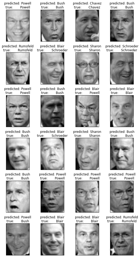
In our second table here, we have printed a confusion matrix, which provides a nice summary visualization of our results: Each row is the actual class, and the columns are the predicted class. For example, in row 1 there are 17 correct identifications of Arial Sharon, and 5 wrong ones. Using our previously defined helper plotting function, we show some examples of predicted vs true names below. Our simple algorithm’s accuracy is imperfect, yet satisfying!

#Plot predictions on a portion of the test set
def title(y_pred, y_test, target_names, i):
pred_name = target_names[y_pred[i]].rsplit(' ', 1)[-1]
true_name = target_names[y_test[i]].rsplit(' ', 1)[-1]
return 'predicted: %s\ntrue: %s'%(pred_name, true_name)

prediction_titles = [title(y_pred, y_test, target_names, i)
for i in range(y_pred.shape[0])]

plot_gallery(X_test, prediction_titles, h, w, 6, 4)

Discussion

85% average accuracy shows that PCA (Eigenface analysis) can provide accurate face recognition results, given just a modest amount of training data. There are pros and cons to eigenfaces however:

• Pros
  1. Training can be automated.
  2. Once the the eigenfaces are calculated, face recognition can be performed in real time.
  3. Eigenfaces can handle large databases.
• Cons
  1. Sensitive to lighting conditions.
  2. Expression changes are not handled well.
  3. Has trouble when the face angle changes.
  4. Difficult to interpret eigenfaces: Eg, one can’t easily read off from these eye separation distance, etc.

There are more advanced facial recognition methods that take advantage of features special to faces. One example is provided by the Active Appearance Model (AAM), which finds facial features (nose, mouth, etc.), and then identifies relationships between these to carry out identifications. Whatever the approach, the overall methodology is the same for all facial recognition algorithms:

1. Take a labeled set of faces.
2. Extract features from those faces using some method of choice (eg eigenfaces).
3. Train a machine learning model on those features.
4. Extract features from a new face, and predict the identity.

The story doesn’t end with finding faces in photos. Facial recognition is just a subset of machine vision, which is currently being applied widely in industry. For example, Intel and other semiconductor manufactures use machine vision to detect defects in the chips being produced — one application where by-hand (human) analysis is not possible and computers have the upper hand.

Like this post? Share on: Twitter | Facebook | Email

Damien RJ Damien is a highly experienced researcher with a background in clinical and applied research. Like JSL, he got his PhD at UCLA. He has many years of experience working with imaging, and has a particularly strong background in image segmentation, registration, detection, data analysis, and more recently machine learning. He now works as a data-scientist at Square in San Francisco.