Mean shift clustering
Mean shift clustering is a general non-parametric cluster finding procedure — introduced by Fukunaga and Hostetler [1], and popular within the computer vision field. Nicely, and in contrast to the more-well-known K-means clustering algorithm, the output of mean shift does not depend on any explicit assumptions on the shape of the point distribution, the number of clusters, or any form of random initialization.
We describe the mean shift algorithm in some detail in the technical background section at the end of this post. However, its essence is readily explained in a few words: Essentially, mean shift treats the clustering problem by supposing that all points given represent samples from some underlying probability density function, with regions of high sample density corresponding to the local maxima of this distribution. To find these local maxima, the algorithm works by allowing the points to attract each other, via what might be considered a short-ranged “gravitational” force. Allowing the points to gravitate towards areas of higher density, one can show that they will eventually coalesce at a series of points, close to the local maxima of the distribution. Those data points that converge to the same local maxima are considered to be members of the same cluster.
In the next couple of sections, we illustrate application of the algorithm to a couple of problems. We make use of the python package SkLearn, which contains a mean shift implementation. Following this, we provide a quick discussion and an appendix on technical details.
Mean shift clustering in action
In today’s post we will have two examples. First, we will show how to use mean shift clustering to identify clusters of data in a 2D data set. Second, we will use the algorithm to segment a picture based on the colors in the image. To do this we need a handful of libraries from sklearn, numpy, matplotlib, and the Python Imaging Library (PIL) to handle reading in a jpeg image.
import numpy as np
from sklearn.cluster import MeanShift, estimate_bandwidth
from sklearn.datasets.samples_generator import make_blobs
import matplotlib.pyplot as plt
from itertools import cycle
from PIL import Image
Finding clusters in a 2D data set
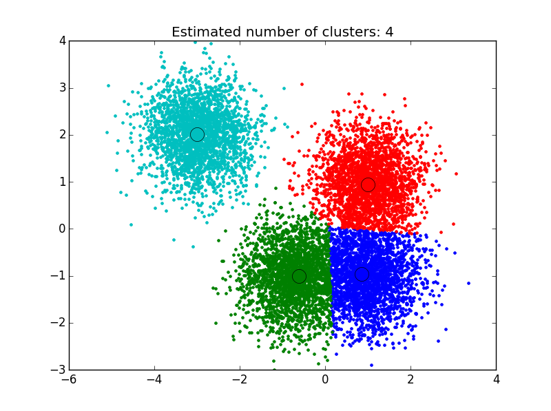
This first example is based off of the sklearn tutorial for mean shift clustering: We generate data points centered at 4 locations, making use of sklearn’s make_blobs library. To apply the clustering algorithm to the points generated, we must first set the attractive interaction length between examples, also know as the algorithm’s bandwidth. Sklearn’s implementation contains a built-in function that allows it to automatically estimate a reasonable value for this, based upon the typical distance between examples. We make use of that below, carry out the clustering, and then plot the results.
#%% Generate sample data
centers = [[1, 1], [-.75, -1], [1, -1], [-3, 2]]
X, _ = make_blobs(n_samples=10000, centers=centers, cluster_std=0.6)

#%% Compute clustering with MeanShift

# The bandwidth can be automatically estimated
bandwidth = estimate_bandwidth(X, quantile=.1,
n_samples=500)
ms = MeanShift(bandwidth=bandwidth, bin_seeding=True)
ms.fit(X)
labels = ms.labels_
cluster_centers = ms.cluster_centers_

n_clusters_ = labels.max()+1

#%% Plot result
plt.figure(1)
plt.clf()

colors = cycle('bgrcmykbgrcmykbgrcmykbgrcmyk')
for k, col in zip(range(n_clusters_), colors):
    my_members = labels == k
    cluster_center = cluster_centers[k]
    plt.plot(X[my_members, 0], X[my_members, 1], col + '.')
    plt.plot(cluster_center[0], cluster_center[1],
    'o', markerfacecolor=col,
    markeredgecolor='k', markersize=14)
plt.title('Estimated number of clusters: %d' % n_clusters_)
plt.show()
As you can see below, the algorithm has found clusters centered on each of the blobs we generated.
Segmenting a color photo
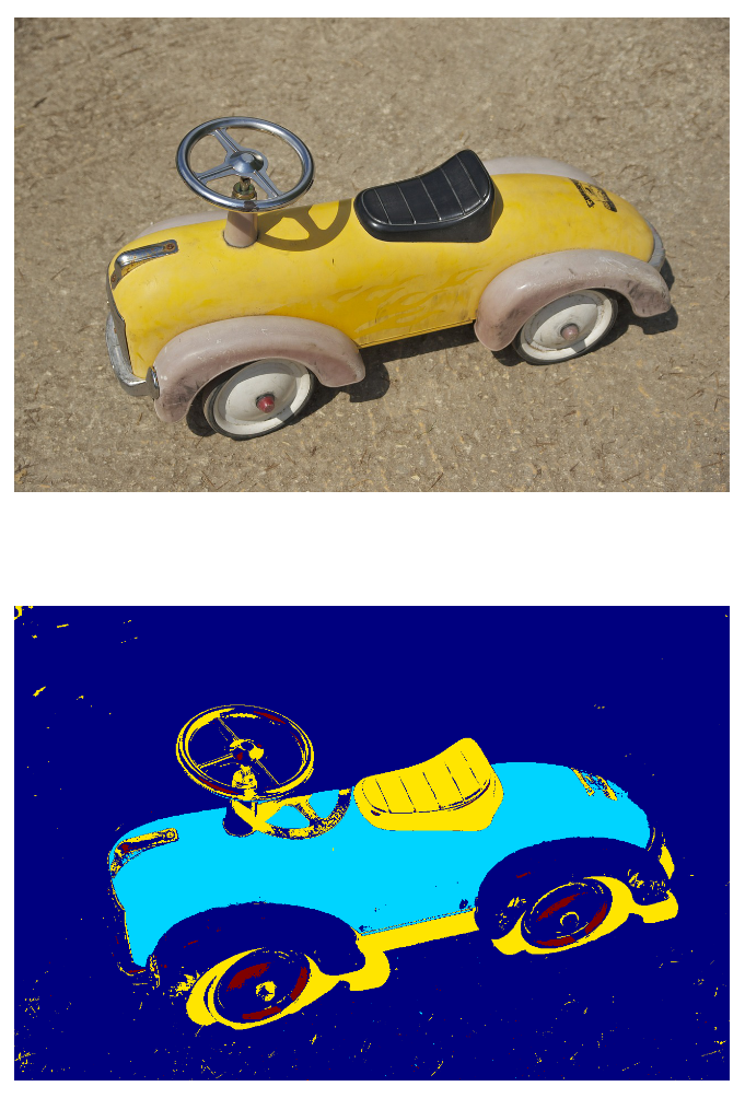
In the first example, we were using mean shift clustering to look for spatial clusters. In our second example, we will instead explore 3D color space, RGB, by considering pixel values taken from an image of a toy car. The procedure is similar — here, we cluster points in 3d, but instead of having data(x,y) we have data(r,g,b) taken from the image’s RGB pixel values. Clustering these color values in this 3d space returns a series of clusters, where the pixels in those clusters are similar in RGB space. Recoloring pixels according to their cluster, we obtain a segmentation of the original image.
#%% Part 2: Color image segmentation using mean shift

image = Image.open('toy.jpg')
image = np.array(image)

#Need to convert image into feature array based
#on rgb intensities
flat_image=np.reshape(image, [-1, 3])

#Estimate bandwidth
bandwidth2 = estimate_bandwidth(flat_image,
quantile=.2, n_samples=500)
ms = MeanShift(bandwidth2, bin_seeding=True)
ms.fit(flat_image)
labels=ms.labels_

# Plot image vs segmented image
plt.figure(2)
plt.subplot(2, 1, 1)
plt.imshow(image)
plt.axis('off')
plt.subplot(2, 1, 2)
plt.imshow(np.reshape(labels, [851,1280]))
plt.axis('off')
The bottom image below illustrates that one can effectively use this approach to identify the key shapes within an image, all without doing any image processing to get rid of glare or background — pretty great!
Discussion
Although mean shift is a reasonably versatile algorithm, it has primarily been applied to problems in computer vision, where it has been used for image segmentation, clustering, and video tracking. Application to big data problems can be challenging due to the fact the algorithm can become relatively slow in this limit. However, research is presently underway to speed up its convergence, which should enable its application to larger data sets.
Mean shift pros:
- No assumptions on the shape or number of data clusters.
- The procedure only has one parameter, the bandwidth.
- Output doesn’t depend on initializations.
Mean shift cons:
- Output does depend on bandwidth: too small and convergence is slow, too large and some clusters may be missed.
- Computationally expensive for large feature spaces.
- Often slower than K-Means clustering
Technical details follow.
Technical background
Kernel density estimation
A general formulation of the mean shift algorithm can be developed through consideration of density kernels. These effectively work by smearing out each point example in space over some small window. Summing up the mass from each of these smeared units gives an estimate for the probability density at every point in space (by smearing, we are able to obtain estimates at locations that do not sit exactly atop any example). This approach is often referred to as kernel density estimation — a method for density estimation that often converges more quickly than binning, or histogramming, and one that also nicely returns a continuous estimate for the density function.
To illustrate, suppose we are given a data set \(\{\textbf{u}_i\}\) of points in d-dimensional space, sampled from some larger population, and that we have chosen a kernel \(K\) having bandwidth parameter \(h\). Together, these data and kernel function return the following kernel density estimator for the full population’s density function
The kernel (smearing) function here is required to satisfy the following two conditions:
- \(\int K(\textbf{u})d\textbf{u} = 1\)
- \(K(\textbf{u})=K(\vert \textbf{u} \vert)\) for all values of \(\textbf{u}\)
The first requirement is needed to ensure that our estimate is normalized, and the second is associated with the symmetry of our space. Two popular kernel functions that satisfy these conditions are given by
- Flat/Uniform \(\begin{align} K(\textbf{u}) = \frac{1}{2}\left\{ \begin{array}{lr} 1 & -1 \le \vert \textbf{u} \vert \le 1\ 0 & else \end{array} \right. \end{align}\)
- Gaussian = \(K(\textbf{u}) = \frac{1}{\left(2\pi\right)^{d/2}} e^{-\frac{1}{2} \vert \textbf{u} \vert^2}\)
Below we plot an example in 1-d using the gaussian kernel to estimate the density of some population along the x-axis. You can see that each sample point adds a small Gaussian to our estimate, centered about it: The equations above may look a bit intimidating, but the graphic here should clarify that the concept is pretty straightforward.
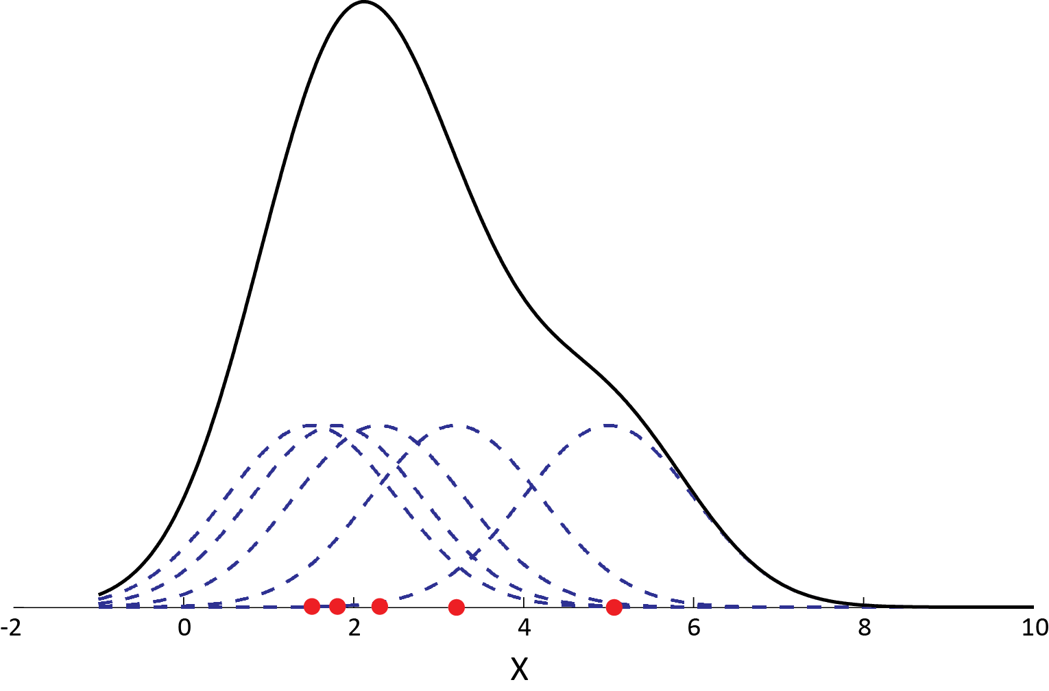 Example of a kernel density estimation using a gaussian kernel for each data point: Adding up small Gaussians about each example returns our net estimate for the total density, the black curve.
Mean shift algorithm
Recall that the basic goal of the mean shift algorithm is to move particles in the direction of local increasing density. To obtain an estimate for this direction, a gradient is applied to the kernel density estimate discussed above. Assuming an angularly symmetric kernel function, \(K(\textbf{u}) = K(\vert \textbf{u} \vert)\), one can show that this gradient takes the form
where
and \(g(\vert \textbf{u} \vert ) = -K'(\vert \textbf{u} \vert)\) is the derivative of the selected kernel profile. The vector \(\textbf{m}(\textbf{u})\) here, called the mean shift vector, points in the direction of increasing density — the direction we must move our example. With this estimate, then, the mean shift algorithm protocol becomes
- Compute the mean shift vector \(\textbf{m}(\textbf{u}_i)\), evaluated at the location of each training example \(\textbf{u}_i\)
- Move each example from \(\textbf{u}_i \to \textbf{u}_i + \textbf{m}(\textbf{u}_i)\)
- Repeat until convergence — ie, until the particles have reached equilibrium.
As a final step, one determines which examples have ended up at the same points, marking them as members of the same cluster.
For a proof of convergence and further mathematical details, see Comaniciu & Meer (2002) [2].
1. Fukunaga and Hostetler, “The Estimation of the Gradient of a Density Function, with Applications in Pattern Recognition”, IEEE Transactions on Information Theory vol 21 , pp 32-40 ,1975 2. Dorin Comaniciu and Peter Meer, Mean Shift : A Robust approach towards feature space analysis, IEEE Transactions on Pattern Analysis and Machine Intelligence vol 24 No 5 May 2002.
 Damien is a highly experienced researcher with a background in clinical and applied research. Like JSL, he got his PhD at UCLA. He has many years of experience working with imaging, and has a particularly strong background in image segmentation, registration, detection, data analysis, and more recently machine learning. He now works as a data-scientist at Square in San Francisco.